pynucastro usage examples

This notebook illustrates some of the higher-level data structures in pynucastro.

[1]:

import pynucastro as pyna

Examining a single rate

There are several ways to load a single rate. If you down load the specific rate file from the JINA ReacLib website, then you can load the rate via load_rate() and just giving that file name, e.g.,

c13pg = pyna.load_rate("c13-pg-n14-nacr")

However, an easier way to do this is to pass in the shorthand name for the rate to a library. Here we’ll read in the entire ReacLib library and get the \({}^{12}\mathrm{C}(\alpha,\gamma){}^{16}\mathrm{O}\) rate. The result will be a Rate object (or an object of a class derived from Rate). There are a lot of methods in the Rate class that allow you to explore the rate.

[2]:

rl = pyna.ReacLibLibrary()
c13pg = rl.get_rate_by_name("c13(p,g)n14")

A Rate can display itself nicely

[3]:

c13pg

[3]:

C13 + p ⟶ N14 + 𝛾

the original reaclib source

we can easily see the original source from ReacLib

[4]:

print(c13pg.original_source)

4
         p  c13  n14                       nacrr     7.55100e+00
 1.518250e+01-1.355430e+01 0.000000e+00 0.000000e+00
 0.000000e+00 0.000000e+00-1.500000e+00
4
         p  c13  n14                       nacrn     7.55100e+00
 1.851550e+01 0.000000e+00-1.372000e+01-4.500180e-01
 3.708230e+00-1.705450e+00-6.666670e-01
4
         p  c13  n14                       nacrr     7.55100e+00
 1.396370e+01-5.781470e+00 0.000000e+00-1.967030e-01
 1.421260e-01-2.389120e-02-1.500000e+00

This is a rate that consists of 3 sets, each of which has 7 coefficients in a form:

\[\lambda = \exp \left [ a_0 + \sum_{i=1}^5 a_i T_9^{(2i-5)/3} + a_6 \ln T_9 \right ]\]

evaluate the rate at a given temperature (in K)

This is just the temperature dependent portion of the rate, usually expressed as \(N_A \langle \sigma v \rangle\)

[5]:

c13pg.eval(1.e9)

[5]:

3883.4778216250666

nuclei involved

The nuclei involved are all Nucleus objects. They have members Z and N that give the proton and neutron number

[6]:

print(c13pg.reactants)
print(c13pg.products)

[p, C13]
[N14]

[7]:

r2 = c13pg.reactants[1]

Note that each of the nuclei are a pynucastro Nucleus type

[8]:

type(r2)

[8]:

pynucastro.nucdata.nucleus.Nucleus

[9]:

print(r2.Z, r2.N)

6 7

temperature sensitivity

We can find the temperature sensitivity about some reference temperature. This is the exponent when we write the rate as

\[r = r_0 \left ( \frac{T}{T_0} \right )^\nu\]

.

We can estimate this given a reference temperature, \(T_0\)

[10]:

c13pg.get_rate_exponent(2.e7)

[10]:

16.21089670710968

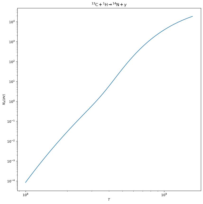
plot the rate’s temperature dependence

A reaction rate has a complex temperature dependence that is defined in the reaclib files. The plot() method will plot this for us

[11]:

fig = c13pg.plot()

density dependence

A rate also knows its density dependence – this is inferred from the reactants in the rate description and is used to construct the terms needed to write a reaction network. Note: since we want reaction rates per gram, this number is 1 less than the number of nuclei

[12]:

c13pg.dens_exp

[12]:

Working with a group of rates

A RateCollection() class allows us to work with a group of rates. This is used to explore their relationship. Other classes (introduced soon) are built on this and will allow us to output network code directly.

Here we create a list with some of the individual rates in the ReacLib library

[13]:

rate_names = ["c12(p,g)n13",
              "c13(p,g)n14",
              "n13(,)c13",
              "n13(p,g)o14",
              "n14(p,g)o15",
              "n15(p,a)c12",
              "o14(,)n14",
              "o15(,)n15"]

rates = rl.get_rate_by_name(rate_names)
rc = pyna.RateCollection(rates=rates)

Printing a rate collection shows all the rates

[14]:

print(rc)

C12 + p ⟶ N13 + 𝛾
C13 + p ⟶ N14 + 𝛾
N13 ⟶ C13 + e⁺ + 𝜈
N13 + p ⟶ O14 + 𝛾
N14 + p ⟶ O15 + 𝛾
N15 + p ⟶ He4 + C12
O14 ⟶ N14 + e⁺ + 𝜈
O15 ⟶ N15 + e⁺ + 𝜈

More detailed information is provided by network_overview()

[15]:

print(rc.network_overview())

p
  consumed by:
     C12 + p ⟶ N13 + 𝛾
     C13 + p ⟶ N14 + 𝛾
     N13 + p ⟶ O14 + 𝛾
     N14 + p ⟶ O15 + 𝛾
     N15 + p ⟶ He4 + C12
  produced by:

He4
  consumed by:
  produced by:
     N15 + p ⟶ He4 + C12

C12
  consumed by:
     C12 + p ⟶ N13 + 𝛾
  produced by:
     N15 + p ⟶ He4 + C12

C13
  consumed by:
     C13 + p ⟶ N14 + 𝛾
  produced by:
     N13 ⟶ C13 + e⁺ + 𝜈

N13
  consumed by:
     N13 ⟶ C13 + e⁺ + 𝜈
     N13 + p ⟶ O14 + 𝛾
  produced by:
     C12 + p ⟶ N13 + 𝛾

N14
  consumed by:
     N14 + p ⟶ O15 + 𝛾
  produced by:
     C13 + p ⟶ N14 + 𝛾
     O14 ⟶ N14 + e⁺ + 𝜈

N15
  consumed by:
     N15 + p ⟶ He4 + C12
  produced by:
     O15 ⟶ N15 + e⁺ + 𝜈

O14
  consumed by:
     O14 ⟶ N14 + e⁺ + 𝜈
  produced by:
     N13 + p ⟶ O14 + 𝛾

O15
  consumed by:
     O15 ⟶ N15 + e⁺ + 𝜈
  produced by:
     N14 + p ⟶ O15 + 𝛾

show a network diagram

We visualize the network using NetworkX. By default, this does not show H or He unless we have H + H or triple-alpha reactions in the network. This is intended to reduce clutter.

[16]:

fig = rc.plot()

There are many options that can be used to configure this plot, for instance, creating a rotated version (useful for very large nets).

Explore the network’s rates

To evaluate the rates, we need a composition

[17]:

comp = pyna.Composition(rc.get_nuclei())
comp.set_solar_like()

Interactive exploration is enabled through the Explorer class, which takes a RateCollection and a Composition

[18]:

re = pyna.Explorer(rc, comp)
re.explore()