Tabulated Weak Rate Example

Here we walk through an example of a single network consisting of just 2 nuclei linked together by electron-capture and beta-decay.

We’ll consider \({}^{56}\mathrm{Ni}\) and \({}^{56}\mathrm{Co}\). The evolution of this system is:

\begin{align*} \frac{dY_\mathrm{Ni}}{dt} &= -\lambda_\mathrm{e-cap} Y_\mathrm{Ni} + \lambda_\mathrm{\beta} Y_\mathrm{Co} \\ \frac{dY_\mathrm{Co}}{dt} &= +\lambda_\mathrm{e-cap} Y_\mathrm{Ni} - \lambda_\mathrm{\beta} Y_\mathrm{Co} \end{align*}

where \(Y_\mathrm{Ni}\) and \(Y_\mathrm{Co}\) are the molar fractions of the nuclei.

Let’s create a network with these rates.

pynucastro will use the tabulated rates from Langanke and Martínez-Pinedo [2001].

import pynucastro as pyna

tl = pyna.TabularLibrary()
lib = tl.linking_nuclei(["ni56", "co56"])
lib

Ni56 + e⁻ ⟶ Co56 + 𝜈           [Q =   2.92 MeV] (Ni56 --> Co56 <tabular_tabular>)
Co56 ⟶ Ni56 + e⁻ + 𝜈           [Q =  -2.92 MeV] (Co56 --> Ni56 <tabular_tabular>)

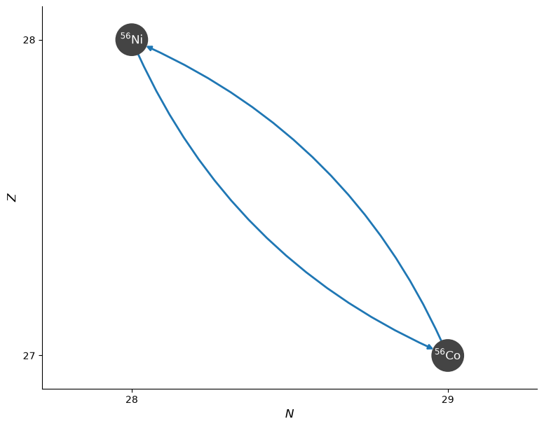
We’ll create a RateCollection so we can evaluate the rates easily

rc = pyna.RateCollection(libraries=[lib])
fig = rc.plot(curved_edges=True)

Let’s create a composition – we’ll make equal amounts of Ni and Co

comp = pyna.Composition(rc.unique_nuclei)
comp.set_equal()

We can see from the electron fraction that we are a little neutron-rich

Ye = comp.eval_ye()
Ye

0.4910714285714286

Now let’s compute the rates. We’ll pick a density (actually \(\rho Y_e\)) and temperature right on one of the points tabulated in the original source so we can directly compare to what is in the table.

rho = 1.e7 / Ye
T = 1.e9

The rates are proportional to the molar fractions, so we can get those too:

Y = comp.get_molar()
Y

{Co56: 0.008928571428571428, Ni56: 0.008928571428571428}

Now we can evaluate the rates

rc.evaluate_rates(rho, T, comp)

{Co56 ⟶ Ni56 + e⁻ + 𝜈: 2.6914293082016787e-23,
 Ni56 + e⁻ ⟶ Co56 + 𝜈: 7.240723730837853e-06}

ydots = rc.evaluate_ydots(rho, T, comp)
ydots

{Co56: 7.240723730837853e-06, Ni56: -7.240723730837853e-06}

If we look at the original tables from Langanke and Martínez-Pinedo [2001], they tabulate (for the conditions we selected above):

 neg. daughter Ni56 z=28 n=28 a=56 Q= -1.6240
 pos. daughter Co56 z=27 n=29 a=56 Q=  1.6240
                      +++ Ni56 --> Co56 +++      --- Co56 --> Ni56 ---
   t9   lrho    uf    lbeta+    leps-    lrnu    lbeta-    leps+  lrnubar
...
  1.00  7.0   0.689  -15.299   -3.091   -3.097  -20.521  -23.856  -20.878
...

We see that there are 2 rates for \({}^{56}\mathrm{Ni} \rightarrow {}^{56}\mathrm{Co}\): positron decay (lbeta+) and electron capture (leps-), and 2 rates for \({}^{56}\mathrm{Co} \rightarrow {}^{56}\mathrm{Ni}\): beta-decay (lbeta-) and positron capture (leps+). All of these are log base-10 in \(\mathrm{s}^{-1}\).

In this case, the dominant rate is the electron capture. Let’s compute that rate manually

lambda_ec = 10.0**-3.091
r = Y[pyna.Nucleus("ni56")] * lambda_ec
r

7.240723730837861e-06

We get the same result as evaluate_rates()!

Finally, we can compute the evolution of the electron fraction:

\[Y_e = \sum_k Z_k Y_k \ \rightarrow \ \frac{dY_e}{dt} = \sum_k Z_k \frac{dY_k}{dt}\]

dyedt = sum(q.Z * ydots[q] for q in rc.unique_nuclei)
dyedt

-7.240723730837865e-06