Approximate Rates

pynucastro can use rate approximations for \(A(\alpha,\gamma)B\) and \(A(\alpha,p)X(p,\gamma)B\), combining them into a single effective rate by assuming that the protons and nucleus \(X\) are in equilibrium.

import pynucastro as pyna
import numpy as np
import matplotlib.pyplot as plt
from scipy.integrate import solve_ivp

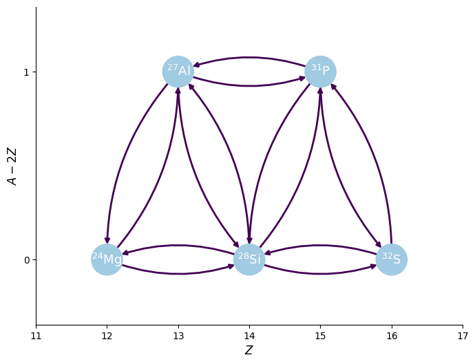
Let’s create a simple network that has both an \((\alpha, \gamma)\) and \((\alpha, p)(p, \gamma)\) sequence.

reaclib_library = pyna.ReacLibLibrary()
mylib = reaclib_library.linking_nuclei(["mg24", "al27", "si28", "p31", "s32", "he4", "p"])
pynet = pyna.PythonNetwork(libraries=[mylib])

fig = pynet.plot(rotated=True, curved_edges=True)

pynet.write_network("full_net.py")

import full_net

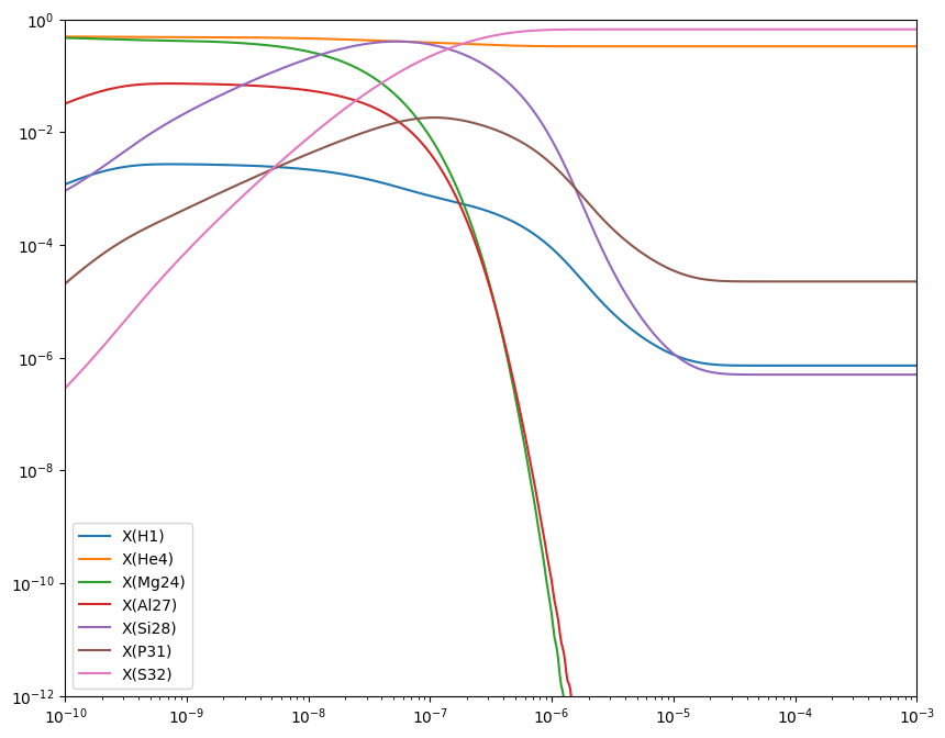
Integrating the full network

Now let’s integrate this. We’ll start with half \({}^{24}\mathrm{Mg}\) and half \(\alpha\) by mass.

rho = 1.e7
T = 3e9

X0 = np.zeros(full_net.nnuc)
X0[full_net.jhe4] = 0.5
X0[full_net.jmg24] = 0.5

Y0 = X0 / full_net.A

tmax = 1.e-3
sol = solve_ivp(full_net.rhs, [0, tmax], Y0, method="BDF",
                dense_output=True, args=(rho, T), rtol=1.e-6, atol=1.e-10)

fig = plt.figure()
ax = fig.add_subplot(111)

for i in range(full_net.nnuc):
    ax.loglog(sol.t, sol.y[i,:] * full_net.A[i], label=f"X({full_net.names[i].capitalize()})")

ax.legend()

ax.set_xlim(1.e-10, 1.e-3)
ax.set_ylim(1.e-12, 1)
fig.set_size_inches((10, 8))

Approximate Version

Now we will approximate the rates, combining \((\alpha, \gamma)\) and \((\alpha, p)(p, \gamma)\) into a single effective rate.

The routine make_ap_pg_approx() will find all of the rates that make up that sequence and create a single ApproximateRate that captures the effective rate. The original rates will still be stored in the ApproximateRate object and will be evaluated to compute the needed approximation when the effective rate is evaluated.

pynet.make_ap_pg_approx()

using approximate rate Mg24 + He4 ⟶ Si28 + 𝛾
using approximate rate Si28 ⟶ Mg24 + He4
using approximate rate Si28 + He4 ⟶ S32 + 𝛾
using approximate rate S32 ⟶ Si28 + He4
removing rate Mg24 + He4 ⟶ Si28 + 𝛾
removing rate Mg24 + He4 ⟶ p + Al27
removing rate Al27 + p ⟶ Si28 + 𝛾
removing rate Si28 ⟶ He4 + Mg24
removing rate Si28 ⟶ p + Al27
removing rate Al27 + p ⟶ He4 + Mg24
removing rate Si28 + He4 ⟶ S32 + 𝛾
removing rate Si28 + He4 ⟶ p + P31
removing rate P31 + p ⟶ S32 + 𝛾
removing rate S32 ⟶ He4 + Si28
removing rate S32 ⟶ p + P31
removing rate P31 + p ⟶ He4 + Si28

pynet

P31 ⟶ He4 + Al27
Al27 + He4 ⟶ P31 + 𝛾
Mg24 + He4 ⟶ Si28 + 𝛾
Si28 ⟶ Mg24 + He4
Si28 + He4 ⟶ S32 + 𝛾
S32 ⟶ Si28 + He4

Since we no longer care about the \({}^{27}\mathrm{Al}\) and \({}^{31}\mathrm{P}\), we can remove them from the network. The ApproximateRate object still knows that these are the intermediate nucleus, but now they won’t explicitly appear as one of the nuclei in the network.

pynet.remove_nuclei(["al27", "p31"])

looking to remove P31 ⟶ He4 + Al27
looking to remove Al27 + He4 ⟶ P31 + 𝛾
looking to remove P31 ⟶ He4 + Al27
looking to remove Al27 + He4 ⟶ P31 + 𝛾

Note that since no reactions consume protons after that removal, the protons are all removed from the network, reducing its size from 7 nuclei to 4

print(pynet.network_overview())

He4
  consumed by:
     Mg24 + He4 ⟶ Si28 + 𝛾
     Si28 + He4 ⟶ S32 + 𝛾
  produced by:
     Si28 ⟶ Mg24 + He4
     S32 ⟶ Si28 + He4

Mg24
  consumed by:
     Mg24 + He4 ⟶ Si28 + 𝛾
  produced by:
     Si28 ⟶ Mg24 + He4

Si28
  consumed by:
     Si28 ⟶ Mg24 + He4
     Si28 + He4 ⟶ S32 + 𝛾
  produced by:
     Mg24 + He4 ⟶ Si28 + 𝛾
     S32 ⟶ Si28 + He4

S32
  consumed by:
     S32 ⟶ Si28 + He4
  produced by:
     Si28 + He4 ⟶ S32 + 𝛾

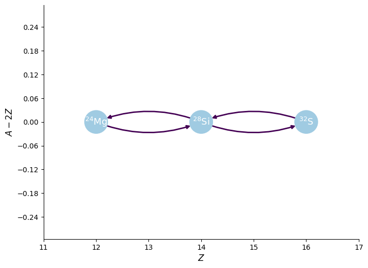
fig = pynet.plot(rotated=True, curved_edges=True)

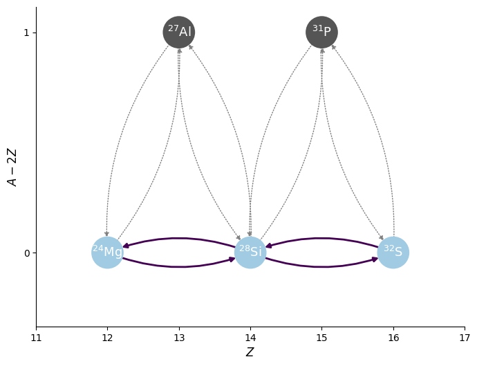
As we see above, the nuclei \({}^{27}\mathrm{Al}\) and \({}^{31}\mathrm{P}\) no longer appear in the network, but the links to them are still understood to the network. This reduces the size of the network, while still preserving those flows.

pynet.write_network("approx_net.py")

import approx_net

The PythonNetwork knows how to write out the code needed to evaluate the rate approximation. For instance, the evolution of \({}^{4}\mathrm{He}\) is determined as:

print(pynet.full_ydot_string(pyna.Nucleus("he4")))

dYdt[jhe4] = (
   -rho*Y[jhe4]*Y[jmg24]*rate_eval.Mg24_He4__Si28__approx
   -rho*Y[jhe4]*Y[jsi28]*rate_eval.Si28_He4__S32__approx
   +Y[jsi28]*rate_eval.Si28__Mg24_He4__approx
   +Y[js32]*rate_eval.S32__Si28_He4__approx
   )

And the rate approximations are computed as:

r = pynet.get_rate("mg24_he4__si28__approx")
print(r.function_string_py())

@numba.njit()
def Mg24_He4__Si28__approx(rate_eval, tf):
    r_ag = rate_eval.He4_Mg24__Si28__removed
    r_ap = rate_eval.He4_Mg24__p_Al27__removed
    r_pg = rate_eval.p_Al27__Si28__removed
    r_pa = rate_eval.p_Al27__He4_Mg24__removed
    rate = r_ag + r_ap * r_pg / (r_pg + r_pa)
    rate_eval.Mg24_He4__Si28__approx = rate

where the 4 lines before the rate approximation is made are evaluating the original, unapproximated rates.

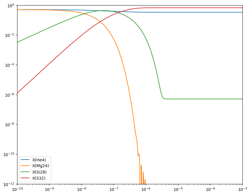
Integrating the approximate network

Let’s integrate this approximate net and compare to above

rho = 1.e7
T = 3.e9

X0 = np.zeros(approx_net.nnuc)
X0[approx_net.jhe4] = 0.5
X0[approx_net.jmg24] = 0.5

Y0 = X0 / approx_net.A

tmax = 1.e-3
approx_sol = solve_ivp(approx_net.rhs, [0, tmax], Y0, method="BDF",
                       dense_output=True, args=(rho, T), rtol=1.e-6, atol=1.e-10)

fig = plt.figure()
ax = fig.add_subplot(111)

for i in range(approx_net.nnuc):
    ax.loglog(approx_sol.t, approx_sol.y[i,:] * approx_net.A[i], label=f"X({approx_net.names[i].capitalize()})")

ax.legend()
ax.set_xlim(1.e-10, 1.e-3)
ax.set_ylim(1.e-12, 1)

fig.set_size_inches((10, 8))

Comparison

Let’s plot both on the same axes to see the comparison.

fig = plt.figure()
ax = fig.add_subplot(111)

for i in range(approx_net.nnuc):
    ax.loglog(approx_sol.t, approx_sol.y[i,:] * approx_net.A[i],
              linestyle=":", color=f"C{i}")

    idx = full_net.names.index(approx_net.names[i])
    ax.loglog(sol.t, sol.y[idx,:] * full_net.A[idx],
              label=f"X({full_net.names[idx].capitalize()})",
              linestyle="-", color=f"C{i}")


ax.legend()
ax.set_xlim(1.e-10, 1.e-3)
ax.set_ylim(1.e-12, 1)

fig.set_size_inches((10, 8))

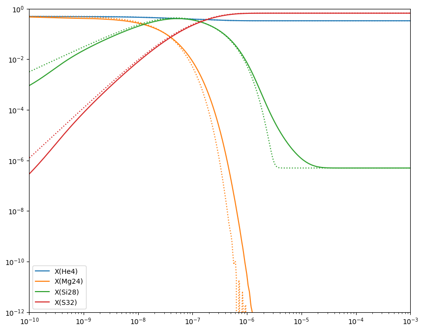
Here the dotted line is the approximate network. We see that the results agree well.

No approximation

What if we just create a 4 nuclei network without the \((\alpha,p)(p,\gamma)\) links? How does this compare?

newlib = reaclib_library.linking_nuclei(["he4", "mg24", "si28", "s32"])
newpynet = pyna.PythonNetwork(libraries=[newlib])
fig = newpynet.plot(rotated=True, curved_edges=True)

newpynet.write_network("simple_net.py")
import simple_net

rho = 1.e7
T = 3e9

X0 = np.zeros(simple_net.nnuc)
X0[simple_net.jhe4] = 0.5
X0[simple_net.jmg24] = 0.5

Y0 = X0 / simple_net.A

simple_net.names == approx_net.names

True

tmax = 1.e-3
simple_sol = solve_ivp(simple_net.rhs, [0, tmax], Y0, method="BDF",
                       dense_output=True, args=(rho, T), rtol=1.e-6, atol=1.e-10)

fig = plt.figure()
ax = fig.add_subplot(111)

for i in range(approx_net.nnuc):
    ax.loglog(approx_sol.t, approx_sol.y[i,:] * approx_net.A[i],
              linestyle=":", color=f"C{i}")

    idx = full_net.names.index(approx_net.names[i])
    ax.loglog(sol.t, sol.y[idx,:] * full_net.A[idx],
              label=f"X({full_net.names[idx].capitalize()})",
              linestyle="-", color=f"C{i}")

    idx = simple_net.names.index(approx_net.names[i])
    ax.loglog(simple_sol.t, simple_sol.y[idx,:] * simple_net.A[idx],
              linestyle="--", color=f"C{i}")


ax.legend()
ax.set_xlim(1.e-10, 1.e-3)
ax.set_ylim(1.e-12, 1)

fig.set_size_inches((10, 8))

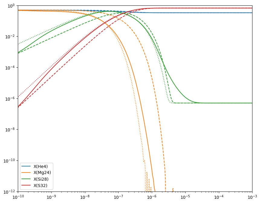
Here we see all 3 networks. The full network (7 nuclei) is the solid lines. The approximate version of that is the dotted line. We see that they track reasonably well, especially when the abundance is high. The dashed line is the version of the network that has the same 4 nuclei as the approximate network, but with out approximating the \((\alpha, p)(p,\gamma)\) links, so we see that the \({}^{24}\mathrm{Mg}\) takes longer to burn.