Integrating Networks with Temperature Evolution

So far, when integrating a reaction network in python, we’ve been solving

\[\frac{d{\bf Y}}{dt} = {\bf f}({\bf Y})\]

where \({\bf f}({\bf Y})\) is provided by the PythonNetwork rhs() function that is generated by write_network.

Now we want to instead solve the system:

\[\frac{d{\bf Y}}{dt} = {\bf f}(T, {\bf Y})\]

\[\frac{dT}{dt} = \frac{\epsilon(T, {\bf Y})}{c_x}\]

where \(\epsilon\) is the specific energy generation rate from the network and \(c_x\) is a specific heat (usually volume or pressure, depending on the application).

Note

The rhs and jacobian functions produced by write_network do not include temperature evolution, so we will need to wrap the rhs function and have the integrator approximate the Jacobian via differencing.

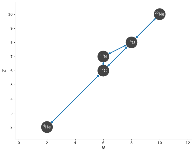
Let’s start with a simple He-burning network.

import pynucastro as pyna

net = pyna.network_helper(["p", "he4", "c12", "n13", "o16", "ne20"])

fig = net.plot()

No temperature evolution

First we’ll integrate without evolving the temperature.

rho = 1.e5
T = 2.e8

comp = pyna.Composition(net.unique_nuclei)
comp.X[pyna.Nucleus("he4")] = 1
comp.normalize()
Y0 = comp.get_molar_array()

tmax = 1.e7

sol = net.integrate_network(tmax, rho, T, Y0, rtol=1.e-6, atol=1.e-6)

/opt/hostedtoolcache/Python/3.14.6/x64/lib/python3.14/site-packages/pynucastro/rates/derived_rate.py:125: UserWarning: C12 partition function is not supported by tables: set log_pf = 0.0 by default
  warnings.warn(UserWarning(f'{nuc} partition function is not supported by tables: set log_pf = 0.0 by default'))
/opt/hostedtoolcache/Python/3.14.6/x64/lib/python3.14/site-packages/pynucastro/rates/derived_rate.py:125: UserWarning: N13 partition function is not supported by tables: set log_pf = 0.0 by default
  warnings.warn(UserWarning(f'{nuc} partition function is not supported by tables: set log_pf = 0.0 by default'))

fig = sol.plot_evolution(ymin=1.e-6)

/opt/hostedtoolcache/Python/3.14.6/x64/lib/python3.14/site-packages/pynucastro/networks/python_network.py:467: UserWarning: Attempt to set non-positive xlim on a log-scaled axis will be ignored.
  ax.set_xlim(tmin, tmax)

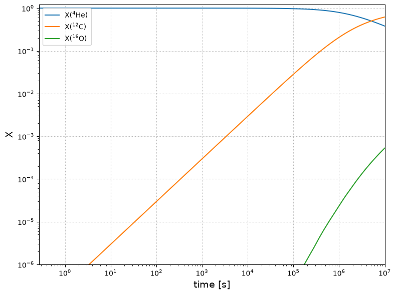
We see it takes about \(10^6\) s for the He mass fraction to start to deplete significantly.

Evolving temperature

When we evolve temperature, we wrap the network’s righthand side function that works on molar fractions, \(Y\), with one that includes temperature. We’ll call our vector of unknowns \(\xi = ({\bf Y}, T)\).

This wrapper that computes \(d\xi/dt\), calling the EOS each evaluation of the righthand side function to get the updated specific heat.

We enable this integration mode by passing self_heating=True to integrate_network.

Note

Currently, temperature support is not present in the Jacobian, so integration with self_heating=True will use a numerical Jacobian. Additionally, the wrapper function is not Numba-compiled. As a result, integrating with temperature evolution can be slow.

sol2 = net.integrate_network(tmax, rho, T, Y0, self_heating=True,
                             rtol=1.e-6, atol=1.e-6)

/opt/hostedtoolcache/Python/3.14.6/x64/lib/python3.14/site-packages/pynucastro/rates/derived_rate.py:125: UserWarning: C12 partition function is not supported by tables: set log_pf = 0.0 by default
  warnings.warn(UserWarning(f'{nuc} partition function is not supported by tables: set log_pf = 0.0 by default'))
/opt/hostedtoolcache/Python/3.14.6/x64/lib/python3.14/site-packages/pynucastro/rates/derived_rate.py:125: UserWarning: N13 partition function is not supported by tables: set log_pf = 0.0 by default
  warnings.warn(UserWarning(f'{nuc} partition function is not supported by tables: set log_pf = 0.0 by default'))

Now we can visualize. First the composition.

fig = sol2.plot_evolution(ymin=1.e-6)

/opt/hostedtoolcache/Python/3.14.6/x64/lib/python3.14/site-packages/pynucastro/networks/python_network.py:467: UserWarning: Attempt to set non-positive xlim on a log-scaled axis will be ignored.
  ax.set_xlim(tmin, tmax)

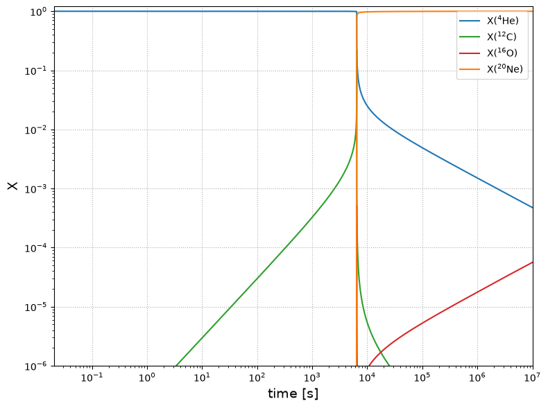
This looks dramatically different than the fixed-temperature case. This is not too surprising, since at these temperatures, the 3-\(\alpha\) rate is very temperature sensitive, so as the temperature increases due to the energy release from burning, the He burning rate increases dramatically.

fig = sol2.plot_temperature()

/opt/hostedtoolcache/Python/3.14.6/x64/lib/python3.14/site-packages/pynucastro/networks/python_network.py:527: UserWarning: Attempt to set non-positive xlim on a log-scaled axis will be ignored.
  ax.set_xlim(tmin, tmax)

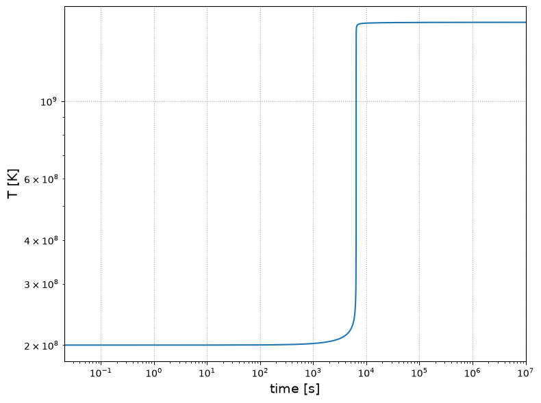
We see that the temperature increased from \(2\times 10^8\) K to over \(1.6\times 10^9\) K.

Caution

In a real star, this energy release would drive a hydrodynamic flow which, depending on the timescale of the energy release vs. sound waves, could drive an expansive flow and quench some of this heating. To really capture this, a full hydrodynamics calculation is needed.

Tip

It is straightforward to include thermal neutrino loses in the temperature evolution equation as well, using the sneut5 method.