Combining ReacLib Rates with Electron Capture Tables

Here’s an example of using tabulated weak rates from Suzuki et al. [2016] together with rates from the ReacLib database.

We’ll build a network suitable for e-capture supernovae.

import pynucastro as pyna

First create a library from ReacLib using a set of nuclei.

reaclib_library = pyna.ReacLibLibrary()

all_nuclei = ["p", "he4",
              "ne20", "o20", "f20",
              "mg24", "al27", "o16",
              "si28", "s32", "p31"]
ecsn_library = reaclib_library.linking_nuclei(all_nuclei,with_reverse=True)

Here are the rates it chose

print(ecsn_library)

O16 + He4 ⟶ Ne20 + 𝛾           [Q =   4.73 MeV] (O16 + He4 --> Ne20 <co10_reaclib__>)
O16 + O16 ⟶ He4 + Si28         [Q =   9.59 MeV] (O16 + O16 --> He4 + Si28 <cf88_reaclib__>)
O16 + O16 ⟶ p + P31            [Q =   7.68 MeV] (O16 + O16 --> p + P31 <cf88_reaclib__>)
O20 ⟶ F20 + e⁻ + 𝜈             [Q =   3.81 MeV] (O20 --> F20 <wc12_reaclib_weak_>)
F20 ⟶ Ne20 + e⁻ + 𝜈            [Q =   7.02 MeV] (F20 --> Ne20 <wc12_reaclib_weak_>)
Ne20 + He4 ⟶ Mg24 + 𝛾          [Q =   9.32 MeV] (Ne20 + He4 --> Mg24 <il10_reaclib__>)
Mg24 + He4 ⟶ Si28 + 𝛾          [Q =   9.98 MeV] (Mg24 + He4 --> Si28 <st08_reaclib__>)
Al27 + p ⟶ He4 + Mg24          [Q =   1.60 MeV] (Al27 + p --> He4 + Mg24 <il10_reaclib__>)
Al27 + p ⟶ Si28 + 𝛾            [Q =  11.59 MeV] (Al27 + p --> Si28 <il10_reaclib__>)
Al27 + He4 ⟶ P31 + 𝛾           [Q =   9.67 MeV] (Al27 + He4 --> P31 <ths8_reaclib__>)
Si28 + He4 ⟶ S32 + 𝛾           [Q =   6.95 MeV] (Si28 + He4 --> S32 <ths8_reaclib__>)
P31 + p ⟶ He4 + Si28           [Q =   1.92 MeV] (P31 + p --> He4 + Si28 <il10_reaclib__>)
P31 + p ⟶ S32 + 𝛾              [Q =   8.86 MeV] (P31 + p --> S32 <il10_reaclib__>)
Ne20 ⟶ He4 + O16               [Q =  -4.73 MeV] (Ne20 --> He4 + O16 <co10_reaclib__reverse>)
Mg24 + He4 ⟶ p + Al27          [Q =  -1.60 MeV] (Mg24 + He4 --> p + Al27 <il10_reaclib__reverse>)
Mg24 ⟶ He4 + Ne20              [Q =  -9.32 MeV] (Mg24 --> He4 + Ne20 <il10_reaclib__reverse>)
Si28 + He4 ⟶ O16 + O16         [Q =  -9.59 MeV] (Si28 + He4 --> O16 + O16 <cf88_reaclib__reverse>)
Si28 + He4 ⟶ p + P31           [Q =  -1.92 MeV] (Si28 + He4 --> p + P31 <il10_reaclib__reverse>)
Si28 ⟶ He4 + Mg24              [Q =  -9.98 MeV] (Si28 --> He4 + Mg24 <st08_reaclib__reverse>)
Si28 ⟶ p + Al27                [Q = -11.59 MeV] (Si28 --> p + Al27 <il10_reaclib__reverse>)
P31 + p ⟶ O16 + O16            [Q =  -7.68 MeV] (P31 + p --> O16 + O16 <cf88_reaclib__reverse>)
P31 ⟶ He4 + Al27               [Q =  -9.67 MeV] (P31 --> He4 + Al27 <ths8_reaclib__reverse>)
S32 ⟶ He4 + Si28               [Q =  -6.95 MeV] (S32 --> He4 + Si28 <ths8_reaclib__reverse>)
S32 ⟶ p + P31                  [Q =  -8.86 MeV] (S32 --> p + P31 <il10_reaclib__reverse>)

Now let’s specify the weak rates we want from Suzuki et al. [2016]. We’ll explicitly use SuzukiLibrary to only consider tabulated rates from that source.

tabular_lib = pyna.SuzukiLibrary()

ecsn_tabular = tabular_lib.linking_nuclei(["f20", "o20", "ne20"])

Let’s look at the rates

tr = ecsn_tabular.get_rates()
tr

[F20 ⟶ Ne20 + e⁻ + 𝜈,
 F20 + e⁻ ⟶ O20 + 𝜈,
 Ne20 + e⁻ ⟶ F20 + 𝜈,
 O20 ⟶ F20 + e⁻ + 𝜈]

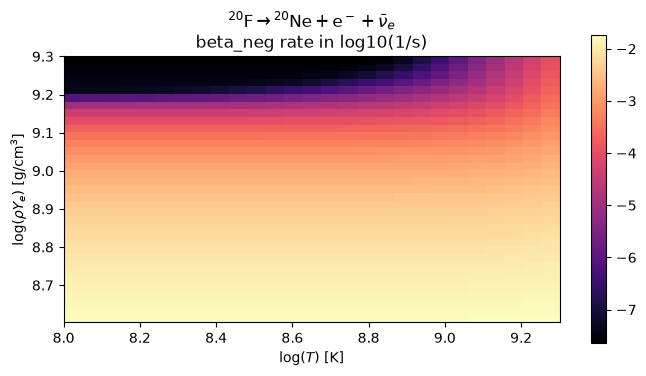
These tables are in terms of \(T\) and \(\rho Y_e\). We can easily plot the tabulated electron capture rates just like ReacLib rates:

fig = tr[0].plot(rhoYmin=4.e8, rhoYmax=2.e9,
                 Tmin=1.e8, Tmax=2.e9,
                 figsize=(8, 4))

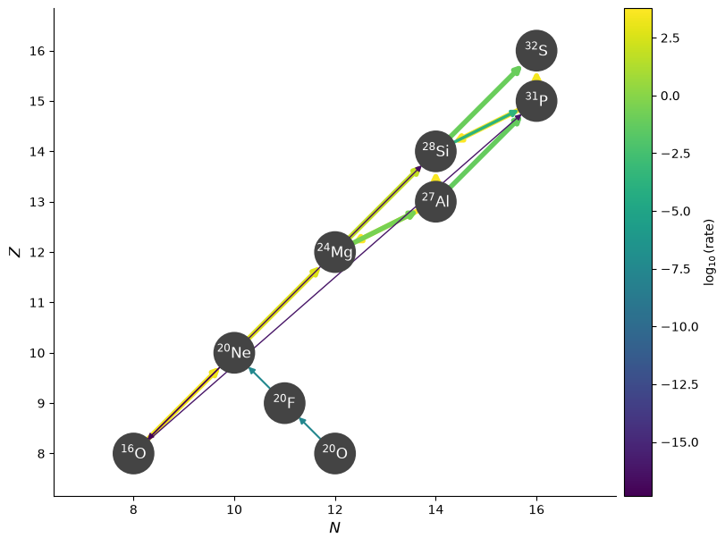
Let’s create a RateCollection from just the ReacLib rates and look to see which are actually important

rc = pyna.RateCollection(libraries=[ecsn_library])

Here we’ll pick thermodynamic conditions appropriate to the oxygen burning shell in a white dwarf

comp = pyna.Composition(rc.get_nuclei())
comp.set_nuc("o16", 0.5)
comp.set_nuc("ne20", 0.3)
comp.set_nuc("mg24", 0.1)
comp.set_nuc("o20", 1.e-5)
comp.set_nuc("f20", 1.e-5)
comp.set_nuc("p", 1.e-5)
comp.set_nuc("he4", 1.e-2)
comp.set_nuc("al27", 1.e-2)
comp.set_nuc("si28", 1.e-2)
comp.set_nuc("s32", 1.e-2)
comp.set_nuc("p31", 1.e-2)
comp.normalize()

fig = rc.plot(rho=7.e9, T=1.e9, comp=comp, ydot_cutoff_value=1.e-20)

Note

This RateCollection already includes some weak rates from ReacLib—we will want to remove those.

We’ll also take the opportunity to remove any rates that are not important, by looking for a \(|\dot{Y}| > 10^{-20}~s^{-1}\). We can use evaluate_rates to help with this.

new_rate_list = []
ydots = rc.evaluate_rates(rho=7.e9, T=1.e9, composition=comp)
for rate in rc.rates:
    if abs(ydots[rate]) >= 1.e-20 and not rate.weak:
        new_rate_list.append(rate)        

Now let’s add the tabular rates to this pruned down rate list

new_rate_list += tr

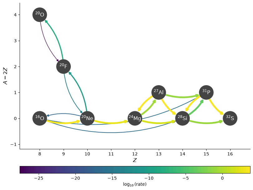
Finally, we’ll create a new RateCollection by combining this new list of rates with the list of tables:

rc_new = pyna.RateCollection(rates=new_rate_list)

fig = rc_new.plot(rho=7.e9, T=1.e9, comp=comp,
                  curved_edges=True, rotated=True)

We can see the values of the rates at our thermodynamic conditions easily:

rc_new.evaluate_rates(rho=7.e9, T=1.e9, composition=comp)

{Ne20 ⟶ He4 + O16: 4.6316695198155e-18,
 O16 + He4 ⟶ Ne20 + 𝛾: 2163.4896055892,
 Ne20 + He4 ⟶ Mg24 + 𝛾: 470.46571662959457,
 Mg24 + He4 ⟶ Si28 + 𝛾: 65.33425925449085,
 Al27 + p ⟶ Si28 + 𝛾: 3786.588954080847,
 Al27 + He4 ⟶ P31 + 𝛾: 0.05763581125914332,
 Si28 + He4 ⟶ S32 + 𝛾: 0.08322738610569612,
 P31 + p ⟶ S32 + 𝛾: 2375.1304964039123,
 O16 + O16 ⟶ p + P31: 7.15493989546395e-17,
 O16 + O16 ⟶ He4 + Si28: 2.5949312230335824e-17,
 Mg24 + He4 ⟶ p + Al27: 0.2543862399303773,
 Al27 + p ⟶ He4 + Mg24: 5920.818449985259,
 Si28 + He4 ⟶ p + P31: 0.00019528201299493384,
 P31 + p ⟶ He4 + Si28: 5491.960442675607,
 F20 ⟶ Ne20 + e⁻ + 𝜈: 1.143049854823845e-14,
 F20 + e⁻ ⟶ O20 + 𝜈: 4.212096660029042e-09,
 Ne20 + e⁻ ⟶ F20 + 𝜈: 4.3100255627801964e-11,
 O20 ⟶ F20 + e⁻ + 𝜈: 2.688308786951095e-28}

Additionally, we can see the specific energy generation rate for these conditions, using evaluate_energy_generation:

rc_new.evaluate_energy_generation(rho=7.e9, T=1.e9, composition=comp)

9.667025588677307e+22