Selecting Rates from a Library

The Library class in pynucastro provides a high level interface for reading files containing one or more Reaclib rates and then filtering these rates based on user-specified criteria for the nuclei involved in the reactions. We can then use the resulting rates to build a network.

Reading a rate snapshot

pynucastro contains that latest ReacLib snapshot and will read that by default.

import pynucastro as pyna

mylibrary = pyna.ReacLibLibrary()

Tip

If the constructor is supplied a file name, pynucastro will read the contents of this file and interpret them as Reaclib rates in either the Reaclib 1 or 2 formats. The Library then stores the rates from the file as Rate objects.

Specifying desired nuclei

This example constructs a CNO network like the one constructed from a set of Reaclib rate files in the pynucastro usage examples section of this documentation.

This time, however, we will specify the nuclei we want in the network and allow the Library class to find all the rates linking only nuclei in the set we specified.

We can specify these nuclei by their abbreviations in the form, e.g. “he4”:

all_nuclei = ["p", "he4", "c12", "n13", "c13", "o14", "n14", "o15", "n15"]

Now we use the Library.linking_nuclei() function to return a smaller Library object containing only the rates that link these nuclei.

Tip

We can pass with_reverse=False to restrict linking_nuclei to only include forward rates from the Reaclib library.

cno_library = mylibrary.linking_nuclei(all_nuclei, with_reverse=False)

Now we can create a network (here we’ll do a PythonNetwork) as:

cno_network = pyna.networks.PythonNetwork(libraries=cno_library)

Note

In the above, we construct a network from a Library object by passing the Library object to the libraries argument of the network constructor. To construct a network from multiple libraries, the libraries argument can also take a list of Library objects.

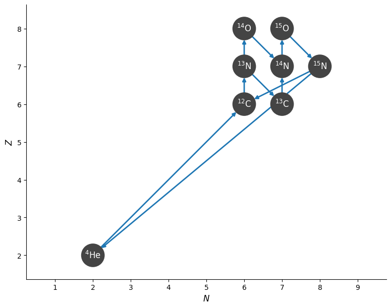
We can show the structure of the network by plotting a network diagram.

fig = cno_network.plot()

Ignoring fixed x limits to fulfill fixed data aspect with adjustable data limits.

Note that the above network also includes the triple-alpha rate from Reaclib.

If we wanted to generate the python code to calculate the right-hand side we could next do:

cno_network.write_network('network_module.py')

And we could run this together with the burn driver program in examples/burn.py

Filtering the library

This example introduces the RateFilter class which allows us to define a set of reactants and products to search for in a Library object.

Inexact filtering

Inexact filtering is like using wildcards: in the following example, the rate filter we define will match any rates in which \(\mathrm{^{12}C}\) is a reactant.

c12_inexact_filter = pyna.RateFilter(reactants=['c12'], exact=False)

Once we construct a RateFilter object, we can apply it to our Library by passing it to the Library.filter function.

Library.filter returns a new Library object containing the rates that match our RateFilter.

We can print a Library to see the rates it contains. In parentheses the rate identifier is printed, showing the Reaclib rate label as well as whether the rate is forward or reverse.

c12_inexact_library = mylibrary.filter(c12_inexact_filter)
print(c12_inexact_library)

C12 + n ⟶ C13 + 𝛾              [Q =   4.95 MeV] (C12 + n --> C13 <ks03_reaclib__>)
C12 + p ⟶ N13 + 𝛾              [Q =   1.94 MeV] (C12 + p --> N13 <ls09_reaclib__>)
C12 + He4 ⟶ O16 + 𝛾            [Q =   7.16 MeV] (C12 + He4 --> O16 <nac2_reaclib__>)
C12 + C12 ⟶ He4 + Ne20         [Q =   4.62 MeV] (C12 + C12 --> He4 + Ne20 <cf88_reaclib__>)
C12 + C12 ⟶ p + Na23           [Q =   2.24 MeV] (C12 + C12 --> p + Na23 <cf88_reaclib__>)
O16 + C12 ⟶ He4 + Mg24         [Q =   6.77 MeV] (O16 + C12 --> He4 + Mg24 <cf88_reaclib__>)
O16 + C12 ⟶ p + Al27           [Q =   5.17 MeV] (O16 + C12 --> p + Al27 <cf88_reaclib__>)
Ne20 + C12 ⟶ He4 + Si28        [Q =  12.02 MeV] (Ne20 + C12 --> He4 + Si28 <rolf_reaclib__>)
Ne20 + C12 ⟶ p + P31           [Q =  10.10 MeV] (Ne20 + C12 --> p + P31 <rolf_reaclib__>)
Ne20 + C12 ⟶ n + S31           [Q =   3.93 MeV] (Ne20 + C12 --> n + S31 <rolf_reaclib__>)
C12 + n ⟶ He4 + Be9            [Q =  -5.70 MeV] (C12 + n --> He4 + Be9 <cf88_reaclib__reverse>)
C12 + n ⟶ p + B12              [Q = -12.59 MeV] (C12 + n --> p + B12 <wag_reaclib__reverse>)
C12 + He4 ⟶ p + N15            [Q =  -4.97 MeV] (C12 + He4 --> p + N15 <nacr_reaclib__reverse>)
C12 + He4 ⟶ n + O15            [Q =  -8.50 MeV] (C12 + He4 --> n + O15 <cf88_reaclib__reverse>)
C12 + C12 ⟶ n + Mg23           [Q =  -2.60 MeV] (C12 + C12 --> n + Mg23 <cf88_reaclib__reverse>)
C12 ⟶ He4 + He4 + He4          [Q =  -7.28 MeV] (C12 --> He4 + He4 + He4 <fy05_reaclib__reverse>)
C12 ⟶ p + B11                  [Q = -15.96 MeV] (C12 --> p + B11 <nw00_reaclib__reverse>)
C12 ⟶ n + C11                  [Q = -18.72 MeV] (C12 --> n + C11 <bb92_reaclib__reverse>)
O16 + C12 ⟶ n + Si27           [Q =  -0.42 MeV] (O16 + C12 --> n + Si27 <cf88_reaclib__reverse>)

The rate identifiers above can be used to access individual Rate objects within a Library as follows:

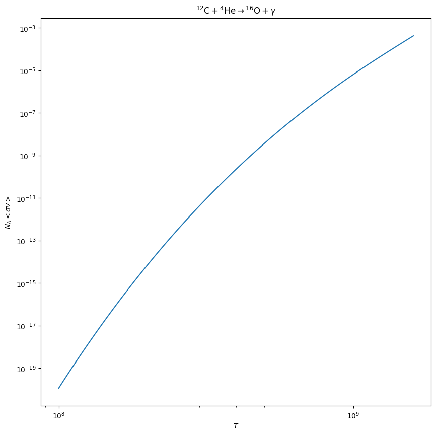
cago = c12_inexact_library.get_rate('c12 + he4 --> o16 <nac2_reaclib__>')

Alternately, we can use the shorthand for a rate

cago = c12_inexact_library.get_rate_by_name("c12(a,g)o16")

fig = cago.plot()

Exact filtering

Exact filtering is useful when you have a specific rate in mind or a specific combination of reactants or products. In the following example, we look for all rates of the form \(\mathrm{^{12}C + ^{12}C \rightarrow \ldots}\)

To use exact filtering, omit the exact keyword to the RateFilter constructor, as it is turned on by default.

Note

Exact filtering does not mean all the nuclei involved in the rate must be specified, it means that all filtering options passed to the RateFilter constructor are strictly applied. In this case, the filter will return rates with exactly two reactants, both of which are \(\mathrm{^{12}C}\). However, the filter places no constraint on the products or number of products in the rate.

c12_exact_filter = pyna.rates.RateFilter(reactants=['c12', 'c12'])
c12_exact_library = mylibrary.filter(c12_exact_filter)
print(c12_exact_library)

C12 + C12 ⟶ He4 + Ne20         [Q =   4.62 MeV] (C12 + C12 --> He4 + Ne20 <cf88_reaclib__>)
C12 + C12 ⟶ p + Na23           [Q =   2.24 MeV] (C12 + C12 --> p + Na23 <cf88_reaclib__>)
C12 + C12 ⟶ n + Mg23           [Q =  -2.60 MeV] (C12 + C12 --> n + Mg23 <cf88_reaclib__reverse>)

Example: building an \(\alpha\)-capture network

In the next example, we use rate filtering to iteratively construct a Library containing the alpha capture rates linking \(\mathrm{^{12}C}\) to \(\mathrm{^{56}Ni}\).

We use the following procedure:

• Start with a seed nucleus, \(\mathrm{^{12}C}\)

• Loop

  • Find the rates that are \(\alpha\)-capture on the current nucleus

  • Use Library.heaviest() to find the heaviest nucleus in the filtered rates. This corresponds to the nucleus with the largest mass number, and in case of a tie between isobars, this returns the isobar with the smallest atomic number.

  • Find the reverse rate using the heaviest nucleus

  • If the mass number of the heaviest nucleus is less that 56, set the seed to the current heaviest nuclei

Note

In the example below, we add each filtered library to our alpha capture library alpha_library, initialized as an empty Library. The Library class supports the addition operator by returning a new library containing the rates in the two libraries we added together.

This example also introduces the max_products keyword, which specifies we are looking for reactions producing at most max_products product nuclei.

Similarly, the RateFilter constructor supports the following keywords constraining the number of reactants and products:

• min_reactants

• max_reactants

• min_products

• max_products

Note

Because we have omitted the argument exact=False, the filter constraints we apply are exact.

alpha_library = pyna.Library()

capture = pyna.Nucleus('he4')
seed = pyna.Nucleus('c12')

while True:
    ac_filter = pyna.RateFilter(reactants=[capture, seed], max_products=1)
    ac_library = mylibrary.filter(ac_filter)
    alpha_library = alpha_library + ac_library

    heavy = ac_library.heaviest()
    ac_filter_inv = pyna.RateFilter(reactants=[heavy], products=[capture, seed])
    ac_inv_library = mylibrary.filter(ac_filter_inv)
    alpha_library = alpha_library + ac_inv_library

    print(heavy)
    if heavy.A == 56:
        break
    else:
        seed = heavy

O16

Ne20

Mg24

Si28

S32

Ar36

Ca40

Ti44

Cr48

Fe52

Ni56

We will next print out the library we constructed, seeing that we have both forward and reverse rates for the alpha chain.

Note that in this example, we are just using the reverse rates provided by ReacLib and not rederiving them via detailed balance together with the nuclear partition function. This can be done using the DerivedRate class.

print(alpha_library)

C12 + He4 ⟶ O16 + 𝛾            [Q =   7.16 MeV] (C12 + He4 --> O16 <nac2_reaclib__>)
O16 + He4 ⟶ Ne20 + 𝛾           [Q =   4.73 MeV] (O16 + He4 --> Ne20 <co10_reaclib__>)
Ne20 + He4 ⟶ Mg24 + 𝛾          [Q =   9.32 MeV] (Ne20 + He4 --> Mg24 <il10_reaclib__>)
Mg24 + He4 ⟶ Si28 + 𝛾          [Q =   9.98 MeV] (Mg24 + He4 --> Si28 <st08_reaclib__>)
Si28 + He4 ⟶ S32 + 𝛾           [Q =   6.95 MeV] (Si28 + He4 --> S32 <ths8_reaclib__>)
S32 + He4 ⟶ Ar36 + 𝛾           [Q =   6.64 MeV] (S32 + He4 --> Ar36 <ths8_reaclib__>)
Ar36 + He4 ⟶ Ca40 + 𝛾          [Q =   7.04 MeV] (Ar36 + He4 --> Ca40 <ths8_reaclib__>)
Ca40 + He4 ⟶ Ti44 + 𝛾          [Q =   5.13 MeV] (Ca40 + He4 --> Ti44 <chw0_reaclib__>)
Ti44 + He4 ⟶ Cr48 + 𝛾          [Q =   7.70 MeV] (Ti44 + He4 --> Cr48 <ths8_reaclib__>)
Cr48 + He4 ⟶ Fe52 + 𝛾          [Q =   7.94 MeV] (Cr48 + He4 --> Fe52 <ths8_reaclib__>)
Fe52 + He4 ⟶ Ni56 + 𝛾          [Q =   8.00 MeV] (Fe52 + He4 --> Ni56 <ths8_reaclib__>)
O16 ⟶ He4 + C12                [Q =  -7.16 MeV] (O16 --> He4 + C12 <nac2_reaclib__reverse>)
Ne20 ⟶ He4 + O16               [Q =  -4.73 MeV] (Ne20 --> He4 + O16 <co10_reaclib__reverse>)
Mg24 ⟶ He4 + Ne20              [Q =  -9.32 MeV] (Mg24 --> He4 + Ne20 <il10_reaclib__reverse>)
Si28 ⟶ He4 + Mg24              [Q =  -9.98 MeV] (Si28 --> He4 + Mg24 <st08_reaclib__reverse>)
S32 ⟶ He4 + Si28               [Q =  -6.95 MeV] (S32 --> He4 + Si28 <ths8_reaclib__reverse>)
Ar36 ⟶ He4 + S32               [Q =  -6.64 MeV] (Ar36 --> He4 + S32 <ths8_reaclib__reverse>)
Ca40 ⟶ He4 + Ar36              [Q =  -7.04 MeV] (Ca40 --> He4 + Ar36 <ths8_reaclib__reverse>)
Ti44 ⟶ He4 + Ca40              [Q =  -5.13 MeV] (Ti44 --> He4 + Ca40 <chw0_reaclib__reverse>)
Cr48 ⟶ He4 + Ti44              [Q =  -7.70 MeV] (Cr48 --> He4 + Ti44 <ths8_reaclib__reverse>)
Fe52 ⟶ He4 + Cr48              [Q =  -7.94 MeV] (Fe52 --> He4 + Cr48 <ths8_reaclib__reverse>)
Ni56 ⟶ He4 + Fe52              [Q =  -8.00 MeV] (Ni56 --> He4 + Fe52 <ths8_reaclib__reverse>)

Next we can create a reaction network from our filtered alpha capture library by passing our library to a network constructor using the libraries keyword.

alpha_network = pyna.PythonNetwork(libraries=alpha_library)

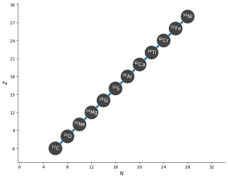
And finally we can make Z-N plot of the nuclei linked via the reactions we selected.

fig = alpha_network.plot()

Ignoring fixed x limits to fulfill fixed data aspect with adjustable data limits.

Note

This is not a realistic network for science applications, because the \((\alpha, p)(p, \gamma)\) links between the nuclei are also important. We’ll discuss adding them (and approximating them) later.