NSE Demonstrations

pynucastro is able to calculate the abundances at nuclear statistical equilibrium (NSE) of a given reaction network.

The constrained equations are setup following Calder et al. [2007] and Seitenzahl et al. [2009] and solved using scipy.optimize.fsolve().

Here we show how to find the NSE state of a set of nuclei.

Creating an NSENetwork

import pynucastro as pyna
import numpy as np
import matplotlib.pyplot as plt
import warnings
warnings.filterwarnings('ignore')

We start by creating a Library object that reads all the ReacLib rates and link different nuclei of choice.

Then initialize NSENetwork by using the the rates created by the Library object.

library = pyna.ReacLibLibrary()

all_nuclei = ["p", "he4",
              "c12", "n13",
              "o16", "ne20", "na23",
              "mg24", "al27", "si28",
              "p31", "s32", "cl35",
              "ar36", "k39", "ca40",
              "sc43", "ti44", "v47",
              "cr48", "mn51",
              "fe52","co55","ni56"]

lib = library.linking_nuclei(all_nuclei)

nse = pyna.NSENetwork(libraries=lib)

We seek the NSE composition at a specified thermodynamic state, the NSENetwork solves the constraint equations for the proton and neutron chemical potentials. Then using this solution, it can compute the mass fractions. The main interface for this is get_comp_nse(rho, T, ye) which returns the composition at NSE as a Composition object.

get_comp_nse() has options of incorporating Coulomb correction terms by setting use_coulomb_corr=True, and to return the proton and neutron chemical potentials by return_sol=True.

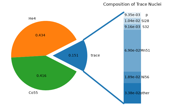
comp, sol = nse.get_comp_nse(1e7, 6e9, 0.50, use_coulomb_corr=True, return_sol=True)
fig = comp.plot()

Tip

There is pre-set initial guess for the proton and neutron chemical potentials, however one should adjust the initial guess, accordingly if no solutions are found or if the method is taking a long time to converge. To pass in the initial guess, set initial_guess=guess, where guess is a user-supplied list of the form [mu_p, mu_n], where mu_p and mu_n are the chemical potential for proton and neutron, respectively.

We can also explicitly print the composition

for c, v in comp.X.items():
    print(f"{str(c):6} : {v:15.8g}")

p      :    0.0093498981
He4    :      0.43364062
C12    :   7.7285996e-06
N13    :   2.5919027e-10
O16    :   1.5697524e-05
Ne20   :   3.0187405e-07
Na23   :   7.2969522e-08
Mg24   :   3.4701942e-05
Al27   :   3.3525822e-05
Si28   :     0.010439163
P31    :    0.0021350073
S32    :    0.0091606019
Cl35   :    0.0040009498
Ar36   :    0.0048794488
K39    :    0.0055527548
Ca40   :    0.0047700285
Sc43   :   0.00037267165
Ti44   :   0.00022927113
V47    :    0.0049046608
Cr48   :    0.0011465823
Mn51   :     0.068958575
Fe52   :    0.0057658969
Co55   :      0.41568674
Ni56   :     0.018915105

print(f"The chemical potential for proton and neutron are {sol[0]:10.7f} and {sol[1]:10.7f}")

The chemical potential for proton and neutron are -7.7387843 and -9.9990481

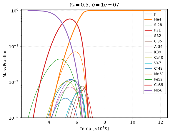
NSE variation with temperature

For \(\rho = 10^7~\mathrm{g~cm^{-3}}\) and electron fraction, \(Y_e = 0.5\), we can explore how the NSE state changes with temperature.

Here we used a guess for chemical potential of proton and neutron of -6.0 and -11.5, respectively.

rho = 1e7
ye = 0.5
temps = np.linspace(2.5, 12.0, 100)
X_s = []

guess = [-6.0, -11.5]
for i, temp in enumerate(temps):
    nse_comp, sol = nse.get_comp_nse(rho, temp*1.0e9, ye, init_guess=guess, 
                                     use_coulomb_corr=True, return_sol=True)
    guess = sol
    nse_X_s = [nse_comp.X[nuc] for nuc in nse_comp.X]
    X_s.append(nse_X_s)

X_s = np.array(X_s)
nuc_names = nse.get_nuclei()

low_limit = 1e-3
fig, ax = plt.subplots()

for k in range(len(nuc_names)):
    lw = 1
    if max(X_s[:, k]) > 0.05:
        lw = 2    
    line, = ax.plot(temps, X_s[:,k], linewidth=lw)
    if (max(X_s[:,k]) > low_limit):
        line.set_label(str(nuc_names[k]))

ax.legend(loc="best", fontsize="small")
ax.set_xlabel(r'Temp $[\times 10^9 K]$')
ax.set_ylabel('Mass Fraction')
ax.set_yscale('log')
ax.set_ylim([low_limit, 1.1])
ax.set_title(rf"$Y_e = {ye}$, $\rho = {rho:6.3g}$")

Text(0.5, 1.0, '$Y_e = 0.5$, $\\rho =  1e+07$')

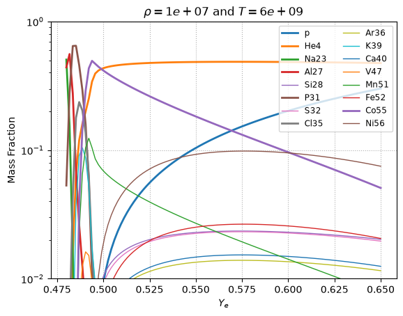
NSE variation with \(Y_e\)

For \(\rho = 10^7~\mathrm{g~cm^{-3}}\) and a relatively high temperature of \(T = 6 \times 10^9~\mathrm{K}\), we can look at how the NSE state changes with varying \(Y_e\).

Note: there will be a lowest \(Y_e\) that is attainable by the network, depending on what species are represented. The NSE configuration with the lowest \(Y_e\) is usually difficult to find and unlikely to happen in reality. For our current example network, achieving the lowest \(Y_e\) means that mass fraction for N13 = 1. As long as protons are in the network, we can reach a \(Y_e\) of \(1\).

ye_low = min(nuc.Z/nuc.A for nuc in nse.unique_nuclei)

rho = 1e7
ye_s = np.linspace(ye_low, 0.65, 100)[1:]
temp = 6.0e9
X_s_1 = []

guess = [-6.0, -11.5]
for i, ye in enumerate(ye_s):
    nse_comp_1, sol = nse.get_comp_nse(rho, temp, ye, init_guess=guess, 
                                       use_coulomb_corr=True, return_sol=True)
    guess = sol
    nse_X_s_1 = [nse_comp_1.X[nuc] for nuc in nse_comp_1.X]
    X_s_1.append(nse_X_s_1)

X_s_1 = np.array(X_s_1)
nuc_names = nse.get_nuclei()

fig, ax = plt.subplots()

for k in range(len(nuc_names)):
    lw = 1
    if max(X_s_1[:, k]) > 0.1:
        lw = 2
    line, = ax.plot(ye_s, X_s_1[:,k], linewidth=lw)
    if (max(X_s_1[:,k]) > 0.01):
        line.set_label(str(nuc_names[k]))

ax.legend(loc="best", fontsize="small", ncol=2)
ax.set_xlabel('ye')
ax.set_ylabel('Mass Fraction')
ax.set_yscale('log')
ax.set_ylim([0.01, 1])
ax.set_title(rf"$\rho = {rho:6.3g}$ and $T={temp:6.3g}$")

Text(0.5, 1.0, '$\\rho =  1e+07$ and $T= 6e+09$')

Comparison with Direct Integration

To further demonstrate the validity of the NSE equation, we will compare the equilibrium mass fractions computed via direct integration and the mass fractions obtained from NSE equations.

We will create the PythonNetwork needed for direct integration using the previously created Library object. To do that we should first modify the previously created Library object so that we use reverse rates calculated via detailed balance. In pynucastro, this is the DerivedRate.

First search through the existing ReacLib reverse rates and remove them. So that Library only contains forward rates

reverse_rates = lib.backward().get_rates()
for r in reverse_rates:
    lib.remove_rate(r)

Now create the corresponding DerivedRate using the forward rate and add them to Library.

for r in lib.get_rates():
    d = pyna.DerivedRate(rate=r, compute_Q=True, use_pf=True)
    lib.add_rate(d)

Now create the PythonNetwork using the modified Library object.

net = pyna.PythonNetwork(libraries=lib)

We can also do some approximations, such as the \((\alpha,p)(p,\gamma)\) approximation. This is fully compatible with NSE.

net.make_ap_pg_approx(intermediate_nuclei=["cl35", "k39", "sc43", "v47", "mn51", "co55"])
net.remove_nuclei(["cl35", "k39", "sc43", "v47", "mn51", "co55"])

using approximate rate S32 + He4 ⟶ Ar36 + 𝛾
using approximate rate Ar36 ⟶ S32 + He4
using approximate rate Ar36 + He4 ⟶ Ca40 + 𝛾
using approximate rate Ca40 ⟶ Ar36 + He4
using approximate rate Ca40 + He4 ⟶ Ti44 + 𝛾
using approximate rate Ti44 ⟶ Ca40 + He4
using approximate rate Ti44 + He4 ⟶ Cr48 + 𝛾
using approximate rate Cr48 ⟶ Ti44 + He4
using approximate rate Cr48 + He4 ⟶ Fe52 + 𝛾
using approximate rate Fe52 ⟶ Cr48 + He4
using approximate rate Fe52 + He4 ⟶ Ni56 + 𝛾
using approximate rate Ni56 ⟶ Fe52 + He4
removing rate S32 + He4 ⟶ Ar36 + 𝛾
removing rate S32 + He4 ⟶ p + Cl35
removing rate Cl35 + p ⟶ Ar36 + 𝛾
removing rate Ar36 ⟶ He4 + S32
removing rate Ar36 ⟶ p + Cl35
removing rate Cl35 + p ⟶ He4 + S32
removing rate Ar36 + He4 ⟶ Ca40 + 𝛾
removing rate Ar36 + He4 ⟶ p + K39
removing rate K39 + p ⟶ Ca40 + 𝛾
removing rate Ca40 ⟶ He4 + Ar36
removing rate Ca40 ⟶ p + K39
removing rate K39 + p ⟶ He4 + Ar36
removing rate Ca40 + He4 ⟶ Ti44 + 𝛾
removing rate Ca40 + He4 ⟶ p + Sc43
removing rate Sc43 + p ⟶ Ti44 + 𝛾
removing rate Ti44 ⟶ He4 + Ca40
removing rate Ti44 ⟶ p + Sc43
removing rate Sc43 + p ⟶ He4 + Ca40
removing rate Ti44 + He4 ⟶ Cr48 + 𝛾
removing rate Ti44 + He4 ⟶ p + V47
removing rate V47 + p ⟶ Cr48 + 𝛾
removing rate Cr48 ⟶ He4 + Ti44
removing rate Cr48 ⟶ p + V47
removing rate V47 + p ⟶ He4 + Ti44
removing rate Cr48 + He4 ⟶ Fe52 + 𝛾
removing rate Cr48 + He4 ⟶ p + Mn51
removing rate Mn51 + p ⟶ Fe52 + 𝛾
removing rate Fe52 ⟶ He4 + Cr48
removing rate Fe52 ⟶ p + Mn51
removing rate Mn51 + p ⟶ He4 + Cr48
removing rate Fe52 + He4 ⟶ Ni56 + 𝛾
removing rate Fe52 + He4 ⟶ p + Co55
removing rate Co55 + p ⟶ Ni56 + 𝛾
removing rate Ni56 ⟶ He4 + Fe52
removing rate Ni56 ⟶ p + Co55
removing rate Co55 + p ⟶ He4 + Fe52
looking to remove P31 + He4 ⟶ Cl35 + 𝛾
looking to remove Cl35 + He4 ⟶ K39 + 𝛾
looking to remove Cl35 ⟶ He4 + P31
looking to remove K39 ⟶ He4 + Cl35
looking to remove Cl35 + He4 ⟶ K39 + 𝛾
looking to remove K39 + He4 ⟶ Sc43 + 𝛾
looking to remove K39 ⟶ He4 + Cl35
looking to remove Sc43 ⟶ He4 + K39
looking to remove K39 + He4 ⟶ Sc43 + 𝛾
looking to remove Sc43 + He4 ⟶ V47 + 𝛾
looking to remove Sc43 ⟶ He4 + K39
looking to remove V47 ⟶ He4 + Sc43
looking to remove Sc43 + He4 ⟶ V47 + 𝛾
looking to remove V47 + He4 ⟶ Mn51 + 𝛾
looking to remove V47 ⟶ He4 + Sc43
looking to remove Mn51 ⟶ He4 + V47
looking to remove V47 + He4 ⟶ Mn51 + 𝛾
looking to remove Mn51 + He4 ⟶ Co55 + 𝛾
looking to remove Mn51 ⟶ He4 + V47
looking to remove Co55 ⟶ He4 + Mn51
looking to remove Mn51 + He4 ⟶ Co55 + 𝛾
looking to remove Co55 ⟶ He4 + Mn51

Now write out python module that contains essential functions needed for integration, such as the rhs and jacobian.

net.write_network(outfile="network.py")

Note

In order for the integrated equilibrium result to be fully compatible with NSE equations, watch out for a number of things:

1. Make sure that all forward rates in the network has a corresponding DerivedRate. Otherwise there is no detailed balance.

2. All species are connected.

3. NSE only guarantees equilibrium of strong reactions. So if there are weak rates in the network, \(Y_e\) will evolve in time.

Now import the network and the screening routine potekhin_1998 and solve using solve_ivp from scipy.integrate

from scipy.integrate import solve_ivp
from pynucastro.screening import potekhin_1998
import network

Set up an initial condition and let it evolve until we reach equilibrium.

rho = 1e7
T = 6e9

X0 = np.ones(network.nnuc)
X0 /= np.sum(X0)
Y0 = X0/network.A

ye = network.ye(Y0)

tmax = 1.e-1
sol = solve_ivp(network.rhs, [0, tmax], Y0, method="BDF",
                 dense_output=True, args=(rho, T, potekhin_1998),
                 rtol=3.e-14, atol=3.e-14, jac=network.jacobian)

Plot to see how mass fraction evolve with time. Equilibrium is indicated by flat lines.

nucs = list(map(pyna.Nucleus, network.names))
nuc_labels = [f"${n.pretty}$" for n in nucs]

fig, ax = plt.subplots()
for i in range(network.nnuc):
    ax.loglog(sol.t, sol.y[i,:]*network.A[i], label=rf"X(${nucs[i].pretty}$)")

ax.set_xlim(1e-16, tmax)
ax.set_xlabel(f"time [s]", fontsize=12)
ax.set_ylabel(f"mass fractions", fontsize=12)
ax.legend(loc="best", fontsize="small", ncol=2)
fig.tight_layout()

Since PythonNetwork used \((\alpha,p)(p,\gamma)\) approximation, do the same for NSENetwork. Then compute the mass fractions predicted from NSE equation.

nse.make_ap_pg_approx(intermediate_nuclei=["cl35", "k39", "sc43", "v47", "mn51", "co55"])
nse.remove_nuclei(["cl35", "k39", "sc43", "v47", "mn51", "co55"])
nse_comp = nse.get_comp_nse(rho, T, ye, init_guess=(-3.5, -14.0), use_coulomb_corr=True)

using approximate rate S32 + He4 ⟶ Ar36 + 𝛾
using approximate rate Ar36 ⟶ S32 + He4
using approximate rate Ar36 + He4 ⟶ Ca40 + 𝛾
using approximate rate Ca40 ⟶ Ar36 + He4
using approximate rate Ca40 + He4 ⟶ Ti44 + 𝛾
using approximate rate Ti44 ⟶ Ca40 + He4
using approximate rate Ti44 + He4 ⟶ Cr48 + 𝛾
using approximate rate Cr48 ⟶ Ti44 + He4
using approximate rate Cr48 + He4 ⟶ Fe52 + 𝛾
using approximate rate Fe52 ⟶ Cr48 + He4
using approximate rate Fe52 + He4 ⟶ Ni56 + 𝛾
using approximate rate Ni56 ⟶ Fe52 + He4
removing rate S32 + He4 ⟶ Ar36 + 𝛾
removing rate S32 + He4 ⟶ p + Cl35
removing rate Cl35 + p ⟶ Ar36 + 𝛾
removing rate Ar36 ⟶ He4 + S32
removing rate Ar36 ⟶ p + Cl35
removing rate Cl35 + p ⟶ He4 + S32
removing rate Ar36 + He4 ⟶ Ca40 + 𝛾
removing rate Ar36 + He4 ⟶ p + K39
removing rate K39 + p ⟶ Ca40 + 𝛾
removing rate Ca40 ⟶ He4 + Ar36
removing rate Ca40 ⟶ p + K39
removing rate K39 + p ⟶ He4 + Ar36
removing rate Ca40 + He4 ⟶ Ti44 + 𝛾
removing rate Ca40 + He4 ⟶ p + Sc43
removing rate Sc43 + p ⟶ Ti44 + 𝛾
removing rate Ti44 ⟶ He4 + Ca40
removing rate Ti44 ⟶ p + Sc43
removing rate Sc43 + p ⟶ He4 + Ca40
removing rate Ti44 + He4 ⟶ Cr48 + 𝛾
removing rate Ti44 + He4 ⟶ p + V47
removing rate V47 + p ⟶ Cr48 + 𝛾
removing rate Cr48 ⟶ He4 + Ti44
removing rate Cr48 ⟶ p + V47
removing rate V47 + p ⟶ He4 + Ti44
removing rate Cr48 + He4 ⟶ Fe52 + 𝛾
removing rate Cr48 + He4 ⟶ p + Mn51
removing rate Mn51 + p ⟶ Fe52 + 𝛾
removing rate Fe52 ⟶ He4 + Cr48
removing rate Fe52 ⟶ p + Mn51
removing rate Mn51 + p ⟶ He4 + Cr48
removing rate Fe52 + He4 ⟶ Ni56 + 𝛾
removing rate Fe52 + He4 ⟶ p + Co55
removing rate Co55 + p ⟶ Ni56 + 𝛾
removing rate Ni56 ⟶ He4 + Fe52
removing rate Ni56 ⟶ p + Co55
removing rate Co55 + p ⟶ He4 + Fe52
looking to remove Cl35 ⟶ He4 + P31
looking to remove K39 ⟶ He4 + Cl35
looking to remove P31 + He4 ⟶ Cl35 + 𝛾
looking to remove Cl35 + He4 ⟶ K39 + 𝛾
looking to remove K39 ⟶ He4 + Cl35
looking to remove Sc43 ⟶ He4 + K39
looking to remove Cl35 + He4 ⟶ K39 + 𝛾
looking to remove K39 + He4 ⟶ Sc43 + 𝛾
looking to remove Sc43 ⟶ He4 + K39
looking to remove V47 ⟶ He4 + Sc43
looking to remove K39 + He4 ⟶ Sc43 + 𝛾
looking to remove Sc43 + He4 ⟶ V47 + 𝛾
looking to remove V47 ⟶ He4 + Sc43
looking to remove Mn51 ⟶ He4 + V47
looking to remove Sc43 + He4 ⟶ V47 + 𝛾
looking to remove V47 + He4 ⟶ Mn51 + 𝛾
looking to remove Mn51 ⟶ He4 + V47
looking to remove Co55 ⟶ He4 + Mn51
looking to remove V47 + He4 ⟶ Mn51 + 𝛾
looking to remove Mn51 + He4 ⟶ Co55 + 𝛾
looking to remove Co55 ⟶ He4 + Mn51
looking to remove Mn51 + He4 ⟶ Co55 + 𝛾

Some plots to see the direct comparison between the two results.

X_net = sol.y[:,-1]*network.A
X_nse = np.array(list(nse_comp.X.values()))

x = np.arange(len(network.names))
width = 0.35

fig, ax = plt.subplots()
ax.bar(x - width/2.0, X_nse, width, label = 'NSE')
ax.bar(x + width/2.0, X_net, width, label = 'Integration')
ax.set_xlabel("nuclei", fontsize=14)
ax.set_xticks(x, labels=nuc_labels, rotation=90, fontsize=14)
ax.set_ylabel("mass fractions", fontsize=14)
ax.legend(fontsize=14)
ax.set_yscale("log")
ax.set_ylim(ymax = 1)
ax.legend()
fig.tight_layout()

Now a plot of absolute and relative difference shows that the mass fraction obtained from direct integration matches with NSE equations to machine precision. The differences between the two are largely set by the tolerances of both the NSE solver and the ODE integrator.

diff = np.abs(X_net - X_nse) 
diff_rel = diff / X_net

fig, ax = plt.subplots()
ax.scatter(x, diff, label='Absolute Error', marker='o', color='r')
ax.scatter(x, diff_rel, label='Relative Error', marker ='x', color='b')
ax.set_xticks(x, labels=nucs, rotation=90, fontsize=14)
ax.set_xlabel("nuclei", fontsize=14)
ax.set_yscale("log")
ax.legend(fontsize=14)
ax.set_ylim(ymax = 1)
ax.legend()
fig.tight_layout()