Creating a Custom Rate#
Let’s imagine wanting to add a rate that has a temperature form not known to pynucastro. We can accomplish this by creating a new class derived from Rate.
We’ll consider a rate of the form:
representing a reaction of the form
then we expect the \(\dot{Y}\) evolution equation for this rate to have the form:
and likewise for the other nuclei.
import pynucastro as pyna
from pynucastro.screening import chugunov_2009
We’ll use this to approximate the rate \({}^{14}\mathrm{N}(p, \gamma){}^{15}\mathrm{O}\) around a temperature of \(T = 3\times 10^7~\mathrm{K}\)
rl = pyna.ReacLibLibrary()
r = rl.get_rate_by_name("n14(p,g)o15")
We can get the values of \(r_0\) and \(\nu\) about this temperature from the rate
T0 = 3.e7
nu = r.get_rate_exponent(T0)
r0 = r.eval(T0)
print(r0, nu)
1.416655077954945e-13 15.601859314950396
Now we can write our custom rate. A few bits are needed in the initialization:
We need to set the “chapter” to “custom”—this will be used by
PythonNetworkto know how to group this rate with the othersWe call the parent
Rateclass’s__init__()to do all the remaining initialization.
We only write 2 additional methods here:
function_string_pyis used when outputting aPythonNetworkto a.pyfile that can be imported and used for integrationevalis used when evaluating the rate interactively (including when making plots)
class MyRate(pyna.Rate):
    def __init__(self, reactants=None, products=None,
                 r0=1.0, T0=1.0, nu=0):

        # we set the chapter to custom so the network knows how to deal with it
        self.chapter = "custom"

        # call the Rate init to do the remaining initialization
        super().__init__(reactants=reactants, products=products)

        self.r0 = r0
        self.T0 = T0
        self.nu = nu

    def function_string_py(self):
        """return a string containing a python function that computes
        the rate"""
        fstring = ""
        fstring += "@numba.njit()\n"
        fstring += f"def {self.fname}(rate_eval, tf):\n"
        fstring += f"    rate_eval.{self.fname} = {self.r0} * (tf.T9 * 1.e9 / {self.T0} )**({self.nu})\n\n"
        return fstring

    def eval(self, T, *, rho=None, comp=None,
             screen_func=None):
        """Evaluate the rate along with screening correction."""

        r = self.r0 * (T / self.T0)**self.nu

        scor = 1.0
        if screen_func is not None:
            if rho is None or comp is None:
                raise ValueError("rho (density) and comp (Composition) needs to be defined when applying electron screening.")
            scor = self.evaluate_screening(rho, T, comp, screen_func)
        r *= scor
        return r
Now we can create our custom rate
r_custom = MyRate(reactants=[pyna.Nucleus("n14"), pyna.Nucleus("p")],
                  products=[pyna.Nucleus("o15")],
                  r0=r0, T0=T0, nu=nu)
r_custom.fname
'N14_p_to_O15_generic'
Notice that it can write out the function needed to evaluate this rate in a python module
print(r_custom.function_string_py())
@numba.njit()
def N14_p_to_O15_generic(rate_eval, tf):
    rate_eval.N14_p_to_O15_generic = 1.416655077954945e-13 * (tf.T9 * 1.e9 / 30000000.0 )**(15.601859314950396)
Creating a network with our rate#
Now let’s create a network that includes this rate. We’ll base it off of the CNO net, but we’ll leave out the rate that we are approximating.
rate_names = ["c12(p,g)n13",
              "c13(p,g)n14",
              "n13(,)c13",
              "n13(p,g)o14",
              "n15(p,a)c12",
              "o14(,)n14",
              "o15(,)n15"]
rates = rl.get_rate_by_name(rate_names)
Here we’ll add our custom rate to the remaining rates we pulled from ReacLib
pynet = pyna.PythonNetwork(rates=rates+[r_custom])
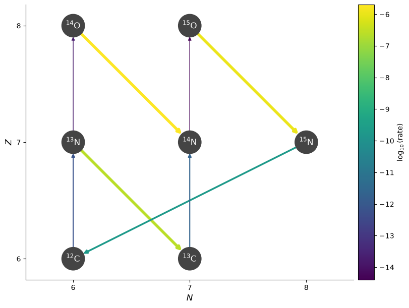
We can plot this to see how it behaves. First a low temperature
T = 3.e7
rho = 200
comp = pyna.Composition(pynet.unique_nuclei)
comp.set_solar_like()
fig = pynet.plot(rho=rho, T=T, comp=comp)
Now a higher temperature and with screening
T = 3.e8
fig = pynet.plot(rho=rho, T=T, comp=comp, screen_func=chugunov_2009)
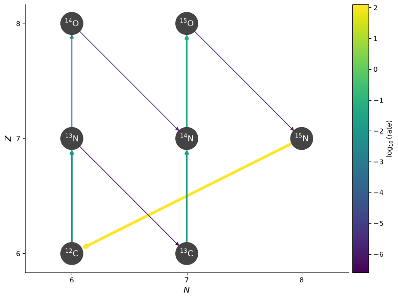
Notice that at the higher temperature, this rate becomes higher than the beta decay to \({}^{13}\mathrm{C}\).
We can also see the values of the ydot terms in the network
pynet.evaluate_ydots(rho, T, comp)
{p: -140.31578946054762,
 He4: 124.10404295119419,
 C12: 124.09500217697241,
 C13: -0.017818574032238365,
 N13: 0.00701794538740977,
 N14: -16.16504349981351,
 N15: -124.1040418689929,
 O14: 0.002020570415053316,
 O15: 16.182863250063768}
Finally, we can see that when the network constructs the dYdt term,
when writing out the network (via write_network), our rate
is included. For example, for the protons:
print(pynet.full_ydot_string(pyna.Nucleus("p")))
dYdt[jp] = (
      -rho*Y[jp]*Y[jc12]*rate_eval.p_C12_to_N13_reaclib  +
      -rho*Y[jp]*Y[jc13]*rate_eval.p_C13_to_N14_reaclib  +
      -rho*Y[jp]*Y[jn13]*rate_eval.p_N13_to_O14_reaclib  +
      -rho*Y[jp]*Y[jn15]*rate_eval.p_N15_to_He4_C12_reaclib  +
      -rho*Y[jp]*Y[jn14]*rate_eval.N14_p_to_O15_generic
   )