A He-burning Network#
Here we create a network that can be used as an \(\alpha\)-chain for modeling He detonations, and includes some of the iron group. It is similar in goals to the classic aprox19 network, but it has some additional rates that are important.
import pynucastro as pyna
Assembling our library#
Core nuclei#
We start with a list of nuclei, including all \(\alpha\)-nuclei up to \({}^{56}\mathrm{Ni}\).
We also add the intermediate nuclei that would participate in \((\alpha,p)(p,\gamma)\) reactions,
as well as a few more nuclei, including those identified by Shen & Bildsten 2009 for bypassing the \({}^{12}\mathrm{C}(\alpha,\gamma){}^{16}\mathrm{O}\) rate. These rates are not present in the classic aprox networks, but can
be very important for the ignition of a detonation.
nuclei = ["p",
          "he4", "c12", "o16", "ne20", "mg24", "si28", "s32",
          "ar36", "ca40", "ti44", "cr48", "fe52", "ni56",
          "al27", "p31", "cl35", "k39", "sc43", "v47", "mn51", "co55",
          "n13", "n14", "f18", "ne21", "na22", "na23"]
For our initial library, we take all of the ReacLib rates that link these.
reaclib_lib = pyna.ReacLibLibrary()
core_lib = reaclib_lib.linking_nuclei(nuclei)
Since we didn’t include neutrons in our list of nuclei, we are missing some potentially important rates, which we now add manually. However, we do not want to carry neutrons, so we modify the endpoints of these reactions, using ModifiedRate to assume
that the original \((X, n)\) reaction is immediately followed by a neutron capture.
other_rates = [("c12(c12,n)mg23", "mg24"),
               ("o16(o16,n)s31", "s32"),
               ("o16(c12,n)si27", "si28")]

for r, mp in other_rates:
    _r = reaclib_lib.get_rate_by_name(r)
    new_rate = pyna.ModifiedRate(_r, new_products=[mp])
    core_lib += pyna.Library(rates=[new_rate])
Iron group#
Next we’ll add some more nuclei in the iron group.
iron_peak = ["n", "p", "he4",
             "mn51",
             "fe52", "fe53", "fe54", "fe55", "fe56",
             "co55", "co56", "co57",
             "ni56", "ni57", "ni58"]
We want to get the rates from both ReacLib and our tabulate weak rate library. Also note that we make sure there is some overlap with the list of nuclei used previously, so these rates will connect to what we already assembled.
iron_reaclib = reaclib_lib.linking_nuclei(iron_peak)

weak_lib = pyna.TabularLibrary()
iron_weak_lib = weak_lib.linking_nuclei(iron_peak)
warning: He4 was not able to be linked in TabularLibrary
warning: Fe53 was not able to be linked in TabularLibrary
warning: Mn51 was not able to be linked in TabularLibrary
warning: Ni58 was not able to be linked in TabularLibrary
warning: Fe52 was not able to be linked in TabularLibrary
warning: Fe54 was not able to be linked in TabularLibrary
Finally, we assemble a Library containing all the rates we selected.
all_lib = core_lib + iron_reaclib + iron_weak_lib
Detailed balance#
We want to replace the reverse rates from ReacLib by rederiving them via detailed balance, and including the partition functions.
rates_to_derive = all_lib.backward().get_rates()

# now for each of those derived rates, look to see if the pair exists

for r in rates_to_derive:
    fr = all_lib.get_rate_by_nuclei(r.products, r.reactants)
    if fr:
        all_lib.remove_rate(r)
        d = pyna.DerivedRate(source_rate=fr, use_pf=True, use_unreliable_spins=True)
        all_lib.add_rate(d)
Removing duplicates#
There will be some duplicate rates now because we pulled rates both from ReacLib and from tabulated sources. Here we keep the tabulated version of any duplicate rates.
all_lib.eliminate_duplicates()
Creating the network#
Now that we have our library, we can make a network. This can be a RateCollection, PythonNetwork, or AmrexAstroCxxNetwork.
Note
For a SimpleCxxNetwork or FortranNetwork, we do not currently support partition functions, so we would need to comment out the above cell that rederives the reverse rates via detailed balance.
net = pyna.PythonNetwork(libraries=[all_lib])
Rate approximations#
Next, we will do the \((\alpha,p)(p,\gamma)\) approximation and eliminate the intermediate nuclei
net.make_ap_pg_approx(intermediate_nuclei=["cl35", "k39", "sc43", "v47"])
net.remove_nuclei(["cl35", "k39", "sc43", "v47"])
We will also approximate some of the neutron captures:
net.make_nn_g_approx(intermediate_nuclei=["fe53", "fe55", "ni57"])
net.remove_nuclei(["fe53", "fe55", "ni57"])
and finally, make some of the protons into NSE protons
net.make_nse_protons(48)
Final stats#
The final network has a variety of different rates supported by pynucastro
net.summary()
Network summary
---------------
  explicitly carried nuclei: 31
  approximated-out nuclei: 7
  inert nuclei (included in carried): 0

  NSE compatible? False

  total number of rates: 154

  rates explicitly connecting nuclei: 115
  hidden rates: 39

  reaclib rates: 67
  starlib rates: 0
  temperature tabular rates: 0
  weak tabular rates: 6
  approximate rates: 14
  derived rates: 64
  modified rates: 3
  custom rates: 0
In all, there are 31 nuclei, but with the approximations, this behaves like a 38-nuclei network.
Visualizing the network#
Let’s visualize the network
fig = net.plot(rotated=True,
               size=(1500, 550),
               node_size=550, node_font_size=11)
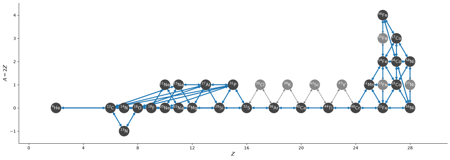
We see a basic \(\alpha\)-network with a few additional nuclei and then a small iron-group NSE set of nuclei.
Test integration#
We’ll write out the network to a python module and do a test integration with it.
net.write_network("he_burn.py")
/opt/hostedtoolcache/Python/3.14.6/x64/lib/python3.14/site-packages/pynucastro/rates/derived_rate.py:125: UserWarning: C12 partition function is not supported by tables: set log_pf = 0.0 by default
  warnings.warn(UserWarning(f'{nuc} partition function is not supported by tables: set log_pf = 0.0 by default'))
/opt/hostedtoolcache/Python/3.14.6/x64/lib/python3.14/site-packages/pynucastro/rates/derived_rate.py:125: UserWarning: N13 partition function is not supported by tables: set log_pf = 0.0 by default
  warnings.warn(UserWarning(f'{nuc} partition function is not supported by tables: set log_pf = 0.0 by default'))
/opt/hostedtoolcache/Python/3.14.6/x64/lib/python3.14/site-packages/pynucastro/rates/derived_rate.py:125: UserWarning: N14 partition function is not supported by tables: set log_pf = 0.0 by default
  warnings.warn(UserWarning(f'{nuc} partition function is not supported by tables: set log_pf = 0.0 by default'))
import he_burn
from scipy.integrate import solve_ivp
import numpy as np
We’ll pick very high temperature and density conditions. At these conditions, electron-captures should be important.
We’ll also set the initial composition to be mostly He with some C–this has \(Y_e = 0.5\) initially.
rho = 5.e8
T = 6.e9

X0 = np.zeros(he_burn.nnuc)
X0[he_burn.jhe4] = 0.95
X0[he_burn.jc12] = 0.05

Y0 = X0/he_burn.A
We’ll include screening in the network
from pynucastro.screening import chugunov_2007
tmax = 1.0

sol = solve_ivp(he_burn.rhs, [0, tmax], Y0, method="BDF", jac=he_burn.jacobian,
                dense_output=True, args=(rho, T, chugunov_2007),
                rtol=1.e-6, atol=1.e-8)
and check if we were successful
sol.success
True
Species evolution#
We can plot the evolution of \(X\) with time.
import matplotlib.pyplot as plt
Here we only plot the most abundant species.
fig, ax = plt.subplots()

for i in range(he_burn.nnuc):
    max_X = sol.y[i, :].max() * he_burn.A[i]
    lw = 1
    ls = "--"
    if max_X > 0.5:
        lw = 2
        ls = "-"
    elif max_X > 0.01:
        lw = 1
        ls = "-"
    if max_X > 5.e-3:
        ax.loglog(sol.t, sol.y[i,:] * he_burn.A[i], lw=lw, ls=ls,
                  label=f"X({he_burn.names[i].capitalize()})")

ax.set_ylim(1.e-6, 1.1)
ax.legend(fontsize="small", ncol=3, loc=3)
ax.set_xlabel("t (s)")
ax.set_ylabel("X")
ax.grid(ls=":")
ax.margins(0)
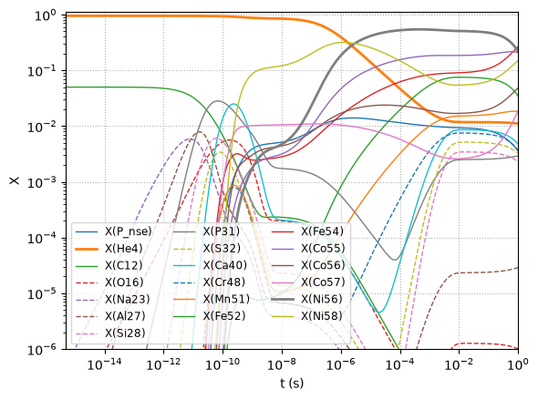
At the very end, we see that the electron-captures on \({}^{56}\mathrm{Ni}\) are starting to decrease its abundance appreciably.
Network flow#
We can also show the flow through the network at the final time.
Xs = sol.y[:, -1] * he_burn.A
comp = pyna.Composition(net.unique_nuclei)
comp.set_array(Xs)
fig = net.plot(rho, T, comp,
               screen_func=chugunov_2007,
               rotated=True,
               color_nodes_by_abundance=True,
               size=(1500, 550),
               ydot_cutoff_value=1.e-20,
               use_net_rate=True,
               Z_range=(1, 29),
               node_size=550, node_font_size=11)
/opt/hostedtoolcache/Python/3.14.6/x64/lib/python3.14/site-packages/pynucastro/rates/derived_rate.py:125: UserWarning: C12 partition function is not supported by tables: set log_pf = 0.0 by default
  warnings.warn(UserWarning(f'{nuc} partition function is not supported by tables: set log_pf = 0.0 by default'))
/opt/hostedtoolcache/Python/3.14.6/x64/lib/python3.14/site-packages/pynucastro/rates/derived_rate.py:125: UserWarning: N13 partition function is not supported by tables: set log_pf = 0.0 by default
  warnings.warn(UserWarning(f'{nuc} partition function is not supported by tables: set log_pf = 0.0 by default'))
/opt/hostedtoolcache/Python/3.14.6/x64/lib/python3.14/site-packages/pynucastro/rates/derived_rate.py:125: UserWarning: N14 partition function is not supported by tables: set log_pf = 0.0 by default
  warnings.warn(UserWarning(f'{nuc} partition function is not supported by tables: set log_pf = 0.0 by default'))
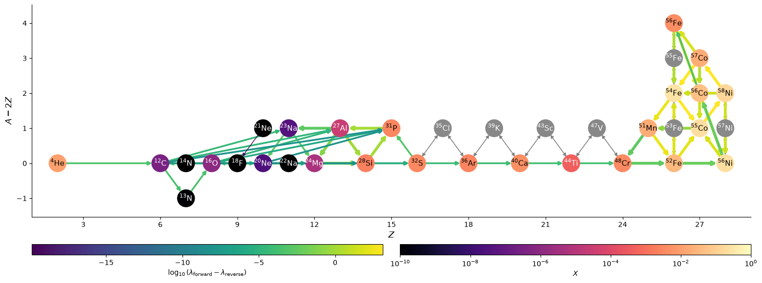
At this point we see that we are really in the iron-group, with some lingering He.
\(Y_e\) evolution#
We also see that the electron captures have decreased our \(Y_e\) a bit:
print(f"Ye = {comp.ye:6.3f}")
Ye = 0.491