hot-CNO and breakout#
We want to explore how the CNO cycle changes as temperature increases and the proton capture rates start becoming much faster. We’ll see that eventually we are limited by \(\beta\)-decays.
import pynucastro as pyna
This collection of rates has the main CNO rates plus a breakout rate into the hot CNO cycle(s)
rl = pyna.ReacLibLibrary()
We’ll get all the rates linking the core nuclei in CNO and the various hot-CNO cycles, but we’ll explicitly remove \(3\)-\(\alpha\), since it is not strong at the temperatures where CNO operates.
linking_nuclei = ["p", "he4",
                  "c12", "c13",
                  "n13", "n14", "n15",
                  "o14", "o15",]
lib = rl.linking_nuclei(linking_nuclei, with_reverse=False)
r3a = lib.get_rate_by_name("he4(aa,g)c12")
lib.remove_rate(r3a)
rc = pyna.RateCollection(libraries=lib)
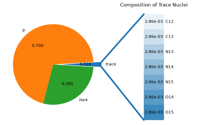
To evaluate the rates, we need a composition. This is defined using a list of Nucleus objects.
Here we set H and He to approximate their solar values and distribute the remaining mass evenly
across the other nuclei.
comp = pyna.Composition(rc.get_nuclei())
comp.set_solar_like()
fig = comp.plot()
Transition from CNO to hot-CNO#
Let’s look at the CNO cycle at a temperature and density just a bit hotter than the Sun’s core
T = 2.e7
rho = 200
fig = rc.plot(rho=rho, T=T, comp=comp, ydot_cutoff_value=1.e-20)
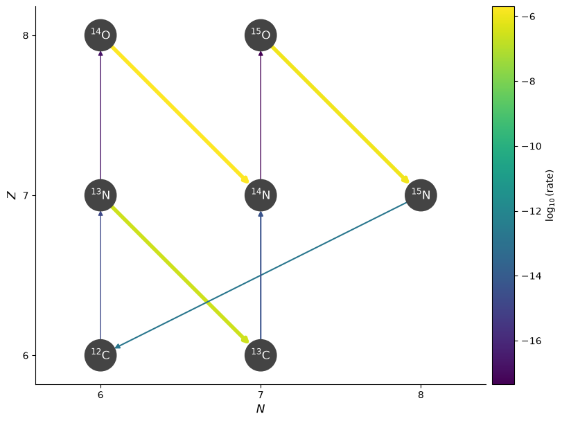
Starting at \({}^{12}\mathrm{C}\), we see the following sequence dominate:
We capture a proton to make \({}^{13}\mathrm{N}\)
\({}^{13}\mathrm{N}\) almost immediately beta decays to \({}^{13}\mathrm{C}\), since the beta-decay rate is so much faster than a proton capture on \({}^{13}\mathrm{N}\).
We continue with proton captures, making \({}^{14}\mathrm{N}\) and then \({}^{15}\mathrm{O}\)
\({}^{15}\mathrm{O}\) then beta-decays to get \({}^{15}\mathrm{N}\)
Finally, one last proton capture, doing \({}^{15}\mathrm{N}(p,\alpha){}^{12}\mathrm{C}\), getting us back to where we started.
This is the basic CNO cycle
Now let’s make it a bit hotter
T = 3.e8
fig = rc.plot(rho=rho, T=T, comp=comp, ydot_cutoff_value=1.e-20)
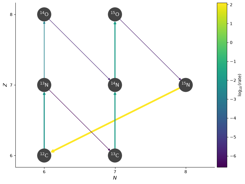
Now we see that the proton capture on \({}^{13}\mathrm{N}\) is faster than the beta-decay, and we make \({}^{14}\mathrm{O}\). Then the cycle continues as before.
As we increase the temperature and density further, we see that the beta decays become the rate-limiting steps.
T = 5.e8
rho = 1.e4
fig = rc.plot(rho=rho, T=T, comp=comp, ydot_cutoff_value=1.e-20)
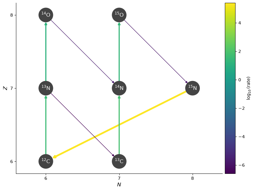
Since the beta-decays are temperature independent (you just have to wait for the nucleus to decay), the overall hot-CNO rate becomes insensitive to temperature.
When does hot-CNO set in?#
We can look at the temperature where we cross from CNO to hot-CNO by looking at the rates involving \({}^{13}\mathrm{N}\)
r1 = rl.get_rate_by_name("n13(p,g)o14")
r2 = rl.get_rate_by_name("n13(,)c13")
import numpy as np
import matplotlib.pyplot as plt
Sample the rates at a range of temperatures
T = np.logspace(7.5, 8.5, 100)

rate_p_capture = [r1.eval(temp) for temp in T]
rate_beta_decay = [r2.eval(temp) for temp in T]
fig, ax = plt.subplots()
ax.loglog(T, rate_p_capture, label=f"{r1.pretty_string}")
ax.loglog(T, rate_beta_decay, label=f"{r2.pretty_string}")
ax.legend()
ax.set_xlabel("T")
ax.set_ylabel(r"$N_A \langle\sigma v\rangle$")
Text(0, 0.5, '$N_A \\langle\\sigma v\\rangle$')
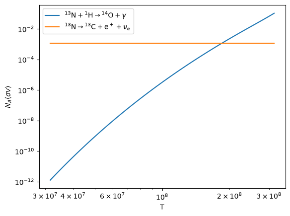
We see that above \(T \sim 2\times 10^8~\mathrm{K}\), the proton-capture proceeds faster than the beta-decay, and we transition to hot-CNO.