Binding Energy per Nucleon

We can explore and plot the binding energy per nucleon to understand when fusion and fission operate.

import pynucastro as pyna

First we’ll get all nuclei with known masses and look at the binding energy

nuclei = pyna.get_all_nuclei()

len(nuclei)

3558

We see there are > 3500 nuclei with measured masses

Most tightly bound nucleus

We can easily find the nucleus that is most tightly bound

nuc_bound = max(nuclei, key=lambda n : n.nucbind)
nuc_bound

Ni62

Binding energy plot

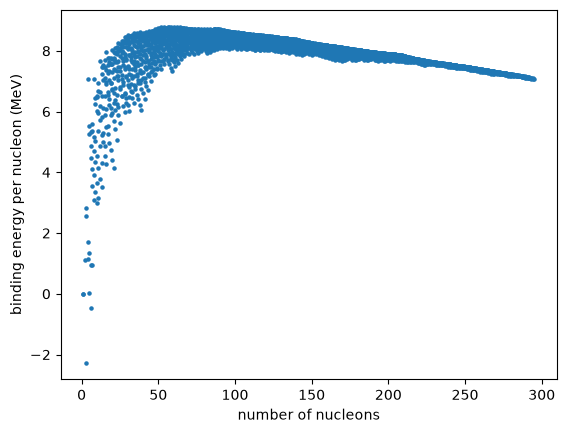
Now we can make a plot of binding energy per nucleon for all nuclei

As = [n.A for n in nuclei]
BEs = [n.nucbind for n in nuclei]

import matplotlib.pyplot as plt

fig, ax = plt.subplots()
ax.scatter(As, BEs, s=5)
ax.set_xlabel("number of nucleons")
ax.set_ylabel("binding energy per nucleon (MeV)")

Text(0, 0.5, 'binding energy per nucleon (MeV)')

Cleaner plot

We see that there is quite a spread in binding energy for each nucleon count. We can instead consider only the most tightly bound nucleus at each mass number. We will also only consider those that are stable (or have half lives > 1 million years)

max_A = max(As)
max_A

295

nuc = []

1 million years in seconds

million_years = 1.e6 * 365.25 * 24 * 3600

for A in range(1, max_A+1):
    # for mass number A, find the nucleus with the maximum binding energy
    try:
        _new = max((n for n in nuclei
                    if n.A == A and (n.tau == "stable" or
                                     (n.tau is not None and n.tau > million_years))),
                   key=lambda q: q.nucbind)
    except ValueError:
        # no stable nucleus of this pass
        continue
    nuc.append(_new)

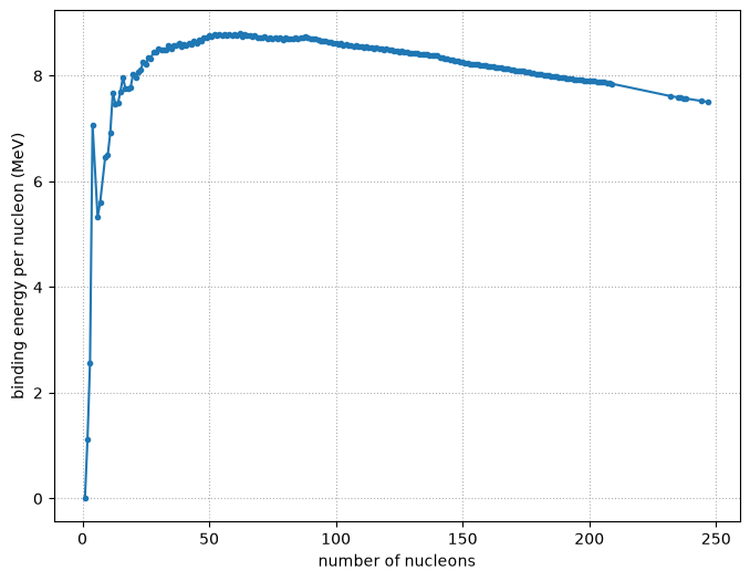
We now plot just these most tightly bound nuclei

As = [n.A for n in nuc]
BEs = [n.nucbind for n in nuc]

fig, ax = plt.subplots()
ax.plot(As, BEs, marker="o", markersize="3")
ax.set_xlabel("number of nucleons")
ax.set_ylabel("binding energy per nucleon (MeV)")
ax.grid(ls=":")
fig.set_size_inches((8, 6))

Visualizing as function of (N, Z)

We want to visualize the mass excess and binding energy in the \(Z\)-\(N\) plane. First let’s get the extent of \(N\) and \(Z\) in our nucleus list.

max_Z = max(nuclei, key=lambda n : n.Z).Z
max_N = max(nuclei, key=lambda n : n.N).N

and the maximum absolute value of the mass excess (in MeV)

dm_mag = abs(max(nuclei, key=lambda n: abs(n.dm)).dm)
dm_mag

201.37

Now we’ll create an array to store dm(Z, N) and be(Z, N) and loop over all the nuclei and store each mass excess and binding energy / nucleon.

import numpy as np
dm = np.zeros((max_Z+1, max_N+1))
be = np.zeros((max_Z+1, max_N+1))

We’ll initialize these to NaN so we can mask out the regions where there are no nuclei

dm[:,:] = np.nan
be[:,:] = np.nan

for n in nuclei:
    dm[n.Z, n.N] = n.dm
    be[n.Z, n.N] = n.nucbind

Note

Due to mass excess estimation in the nuclear databases, a few nuclei have negative binding energies.

n = [n for n in nuclei if n.nucbind < 0]
n

[Li3, B6]

Finally, we can plot

import matplotlib as mpl

# mask out the regions with no nuclei
cmap = mpl.colormaps['RdYlBu']
cmap.set_bad(color='white')

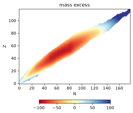
fig, ax = plt.subplots()
im = ax.imshow(dm, origin="lower", cmap="RdYlBu",
               vmin=-100, vmax=100)
ax.set_xlabel("N")
ax.set_ylabel("Z")
ax.set_title("mass excess")
fig.colorbar(im, ax=ax, location="bottom", shrink=0.5)

<matplotlib.colorbar.Colorbar at 0x7fa9b6f87590>

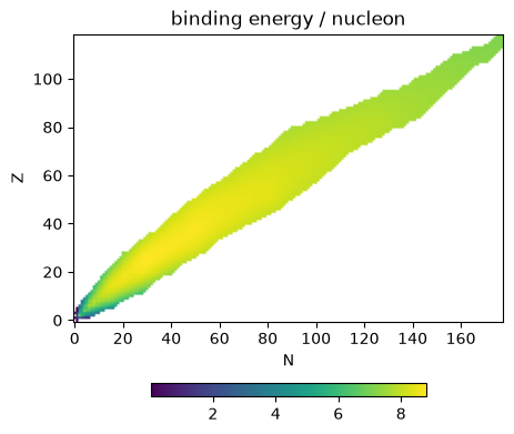
# mask out the regions with no nuclei
cmap = mpl.colormaps['viridis']
cmap.set_bad(color='white')

fig, ax = plt.subplots()
im = ax.imshow(be, origin="lower", cmap=cmap,
               vmin=0.01, vmax=np.nanmax(be))
ax.set_xlabel("N")
ax.set_ylabel("Z")
ax.set_title("binding energy / nucleon")
fig.colorbar(im, ax=ax, location="bottom", shrink=0.5)

<matplotlib.colorbar.Colorbar at 0x7fa9b4908d10>