Approximating double n-capture

We want to approximate the sequence \(A(n,\gamma)X(n,\gamma)B\) as \(A(nn,\gamma)B\) by combining the two successive neutron captures into a single rate, assuming equilibrium of nucleus \(X\).

This type of approximation is commonly done in the “aprox” family of networks, for example, approximating the sequence: \({}^{52}\mathrm{Fe}(n,\gamma){}^{53}\mathrm{Fe}(n,\gamma){}^{54}\mathrm{Fe}\).

import pynucastro as pyna

Unapproximated version

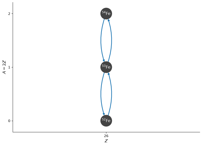
We’ll create a simple network of iron isotopes linked by neutron capture.

rl = pyna.ReacLibLibrary()
lib = rl.linking_nuclei(["fe52", "fe53", "fe54", "n"])

net = pyna.PythonNetwork(libraries=[lib])

fig = net.plot(rotated=True, curved_edges=True)

Now we’ll integrate it, starting with a mix of \({}^{52}\mathrm{Fe}\) and \(n\).

rho = 1.e9
T = 3.e9
comp = pyna.Composition(net.unique_nuclei, small=0.0)
comp.X[pyna.Nucleus("n")] = 0.5
comp.X[pyna.Nucleus("Fe52")] = 0.5
Y0 = comp.get_molar_array()

tmax = 1.e-11

sol = net.integrate_network(tmax, rho, T, Y0, rtol=1.e-6, atol=1.e-8)

fig = sol.plot_evolution(ymin=1.e-6)

/opt/hostedtoolcache/Python/3.14.5/x64/lib/python3.14/site-packages/pynucastro/networks/python_network.py:407: UserWarning: Attempt to set non-positive xlim on a log-scaled axis will be ignored.
  ax.set_xlim(tmin, tmax)

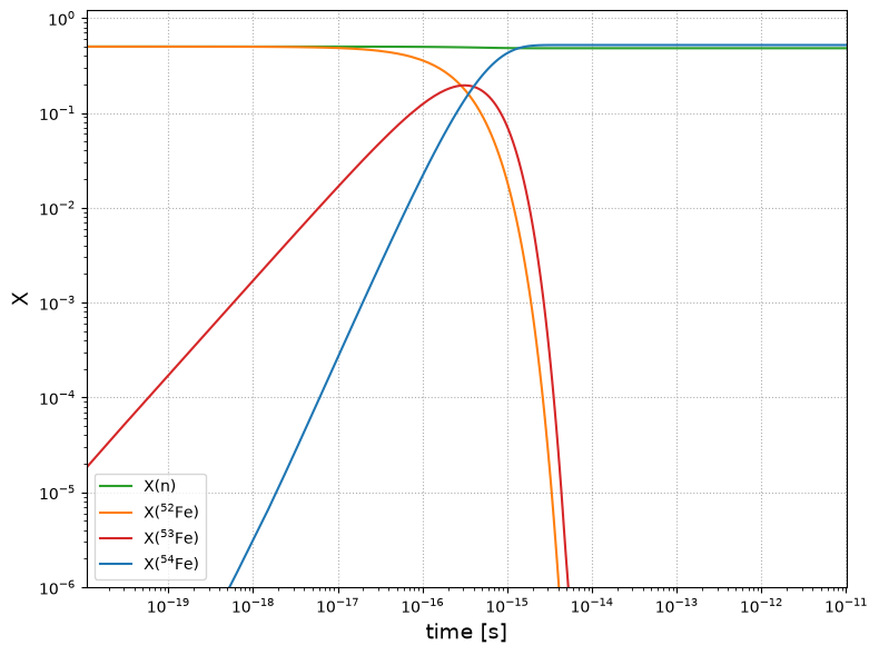
We see that the long term evolution is that all the iron winds up as \({}^{54}\mathrm{Fe}\).

Approximating the double n capture

We can use the helper function create_double_neutron_capture() to create a pair (forward and reverse) of ApproximateRates that approximate out the intermediate nucleus:

rf, rr = pyna.rates.create_double_neutron_capture(rl, pyna.Nucleus("fe52"), pyna.Nucleus("fe54"))

rf

Fe52 + n + n ⟶ Fe54 + 𝛾

We can see what rates this carries internally:

rf.hidden_rates

[Fe52 + n ⟶ Fe53 + 𝛾, Fe53 + n ⟶ Fe54 + 𝛾, Fe54 ⟶ n + Fe53, Fe53 ⟶ n + Fe52]

Tip

Alternately, we could use the make_nn_g_approx() method on the PythonNetwork once we create it.

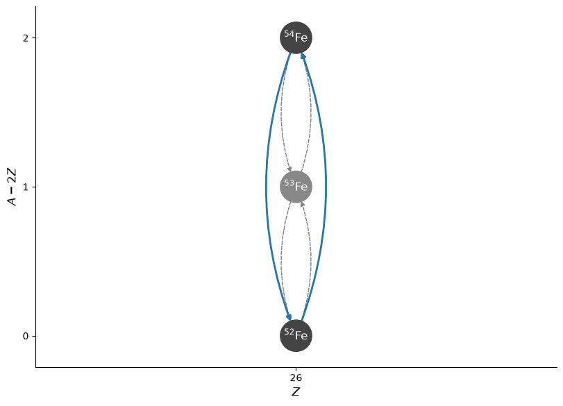
Now we’ll build a new network with just these approximate rates:

net_approx = pyna.PythonNetwork(rates=[rf, rr])

fig = net_approx.plot(rotated=True, curved_edges=True)

comp = pyna.Composition(net_approx.unique_nuclei, small=0.0)
comp.X[pyna.Nucleus("n")] = 0.5
comp.X[pyna.Nucleus("Fe52")] = 0.5
Y0 = comp.get_molar_array()

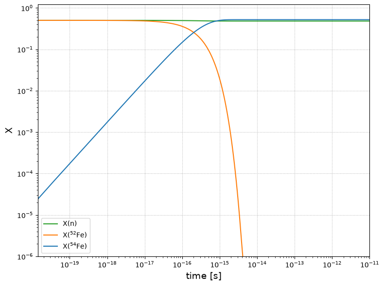
sol_approx = net_approx.integrate_network(tmax, rho, T, Y0, rtol=1.e-6, atol=1.e-8)

fig = sol_approx.plot_evolution(ymin=1.e-6)

/opt/hostedtoolcache/Python/3.14.5/x64/lib/python3.14/site-packages/pynucastro/networks/python_network.py:407: UserWarning: Attempt to set non-positive xlim on a log-scaled axis will be ignored.
  ax.set_xlim(tmin, tmax)

Comparison

Finally, let’s plot the nuclei in common from both nets together

import matplotlib.pyplot as plt

fig, ax = plt.subplots()

for i, nuc in enumerate(sol_approx.unique_nuclei):
    ax.loglog(sol_approx.t, sol_approx.X[i, :],
              linestyle=":", color=f"C{i}")    
    idx = sol.unique_nuclei.index(nuc)
    ax.loglog(sol.t, sol.X[idx, :],
              label=rf"X$({nuc.pretty})$",              
              linestyle="-", color=f"C{i}")

ax.set_ylim(1.e-6, 1.1)
ax.set_xlim(1.e-19, 1.e-11)
ax.set_xlabel("time (s)")
ax.set_ylabel("X")
ax.legend()
ax.grid(ls=":")

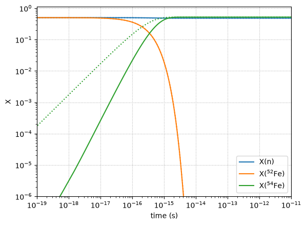
Here the dotted line is the approximate version. We see that the \({}^{52}\mathrm{Fe}\) is consumed at the same rate. The approximate net produces \({}^{54}\mathrm{Fe}\) faster simply because there is no intermediate \({}^{53}\mathrm{Fe}\) in the network.