Using NSE Protons#
A common approximation done in networks is to split the protons into 2 groups, with one group restricted to participating in the iron-group photo-ionization rates / NSE. This is done,
for example, in the common aprox19 and aprox21 networks (see Weaver et al. 1978).
This decouples the proton links for the low-\(A\) and high-\(A\) nuclei, making the linear algebra and network integration easier.
pynucastro supports this approximation at the network level through the make_nse_protons() method.
Test Network#
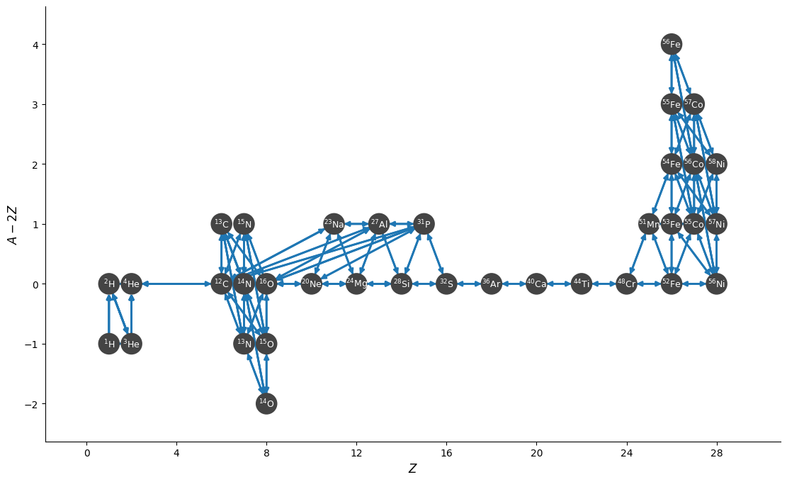
Here we construct a simple example of an H-He network with some iron group.
Caution
This example is not intended to be used as a production network – it is missing weak rates, and \((\alpha,p)(p,\gamma)\) links – it is simply meant to show how to split the protons into 2 groups.
import pynucastro as pyna
nuclei = ["p", "n", "d", "he3", "he4",
          "c12", "c13", "n13", "n14", "n15",
          "o14", "o15", "o16",
          "ne20", "na23", "mg24", "al27", "p31",
          "si28", "s32", "ar36", "ca40", "ti44",
          "cr48", "mn51",
          "fe52", "fe53", "fe54", "fe55", "fe56",
          "co55", "co56", "co57", "ni56", "ni57", "ni58"]
rl = pyna.ReacLibLibrary()
lib = rl.linking_nuclei(nuclei)
rc = pyna.RateCollection(libraries=lib)
fig = rc.plot(rotated=True, hide_xp=True, hide_xalpha=True,
              node_size=400, node_font_size="9", size=(1100, 700))

len(rc.unique_nuclei)
36
comp = pyna.Composition(rc.unique_nuclei)
comp.set_equal()
rho = 1.e6
T = 2.e9
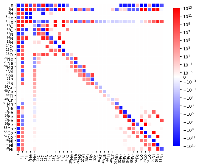
fig = rc.plot_jacobian(rho, T, comp, rate_scaling=1.e16)

From the Jacobian, we can see that the protons are split into two groups, those participating in reactions with \(A \le 32\) and those participating in reactions with \(A \ge 51\).
NSE Protons#
We can split these by adding an “NSE proton”. This evaluates the same as a regular proton, but tests as distinct, allowing the network to have 2 separate protons.
p = pyna.Nucleus("p")
p_nse = pyna.Nucleus("p_NSE")
p, p_nse
(p, p_nse)
p == p_nse
False
p.Z == p_nse.Z
True
p.A == p_nse.A
True
Splitting the Protons in Our Network#
We’ll make all the reactions involving nuclei with \(A \ge 48\) use the NSE protons.
A = 48
rc.make_nse_protons(A)
Note
We need to rebuild the composition, since we now have one additional nucleus
in the network (p_nse).
comp_new = pyna.Composition(rc.unique_nuclei)
comp_new.set_equal()
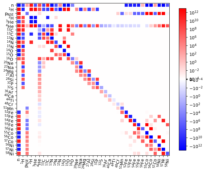
fig = rc.plot_jacobian(rho, T, comp_new, rate_scaling=1.e16)

The Jacobian now shows that the reactions involving heavy nuclei are using p_nse protons, decoupling them from the lower mass nuclei.
