Modified Rates

A ModifiedRate acts as a wrapper, encapsulating a single rate, allowing you to change the products of the stoichiometric coefficients. A good example of this comes from the aprox19 and aprox21 networks. There, an approximation to H-burning (via pp and CNO) is included, and the nucleus \({}^{14}\mathrm{N}\) is present, which is the bottleneck for CNO. Beyond that is an \(\alpha\)-chain. But \(\alpha\)-captures cannot connect \({}^{14}\mathrm{N}\) (odd \(Z\)) to the even-\(Z\) nuclei in the \(\alpha\)-chain.

To make this connection, a rate that does:

\[2\, {}^{14}\mathrm{N} + 3 \alpha \rightarrow 2\, {}^{20}\mathrm{Ne}\]

is added. For a single \({}^{14}\mathrm{N}\) we can write this as \({}^{14}\mathrm{N}(1.5\alpha,\gamma){}^{20}\mathrm{Ne}\). This is assumed to proceed at the rate for \({}^{14}\mathrm{N}(\alpha,\gamma){}^{18}\mathrm{F}\), and \({}^{18}\mathrm{F}\) is not included explicitly in the network. But we can add this approximation using ModifiedRate.

import pynucastro as pyna

We’ll start with a basic network for He burning up to \({}^{20}\mathrm{Ne}\):

rl = pyna.ReacLibLibrary()
lib = rl.linking_nuclei(["he4", "c12", "o16", "ne20"],
                        with_reverse=False)

Now let’s get the \({}^{14}\mathrm{N}(1.5\alpha,\gamma){}^{20}\mathrm{Ne}\) rate and modify it to go to \({}^{20}\mathrm{Ne}\). To do this, we need to change the stoichiometric coefficients as well as the products:

n14rate = rl.get_rate_by_name("n14(a,g)f18")

new_n14 = pyna.ModifiedRate(n14rate,
                            new_products=[pyna.Nucleus("ne20")],
                            stoichiometry={pyna.Nucleus("he4"): 1.5})

new_n14

N14 + 1.5 He4 ⟶ Ne20 + 𝛾

The modified rate still knows the underlying rate we will be evaluating:

new_n14.original_rate

N14 + He4 ⟶ F18 + 𝛾

and we can see that the function to compute the rate simply evaluates the original rate and uses it.

print(new_n14.function_string_py())

@numba.njit()
def He4_N14__Ne20__modified(rate_eval, tf):
    # N14 + 1.5 He4 --> Ne20
    He4_N14__F18(rate_eval, tf)
    rate_eval.He4_N14__Ne20__modified = rate_eval.He4_N14__F18

Now we can add this new rate to our library:

lib.add_rate(new_n14)

and create the network from this library:

net = pyna.PythonNetwork(libraries=[lib])

The evolution for \(dY({}^{4}\mathrm{He})/dt\) also uses the correct coefficient:

print(net.full_ydot_string(pyna.Nucleus("he4")))

dYdt[jhe4] = (
      -rho*Y[jhe4]*Y[jc12]*rate_eval.He4_C12__O16  +
      -rho*Y[jhe4]*Y[jo16]*rate_eval.He4_O16__Ne20  +
      +5.00000000000000e-01*rho*Y[jc12]**2*rate_eval.C12_C12__He4_Ne20  +
      + -3*1.66666666666667e-01*rho**2*Y[jhe4]**3*rate_eval.He4_He4_He4__C12  +
      + -1.5*rho*Y[jhe4]*Y[jn14]*rate_eval.He4_N14__Ne20__modified
   )

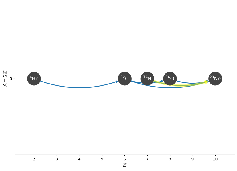
Here’s a visualization with the links from the new rate highlighted:

fig = net.plot(curved_edges=True, rotated=True, hide_xalpha=True,
               highlight_filter_function=lambda r: pyna.Nucleus("n14") in r.reactants)

and the evaluation of the rates at a particular thermodynamic state:

rho = 1.e6
T = 5.e8
comp = pyna.Composition(net.unique_nuclei)
comp.set_equal()

net.evaluate_rates(rho=rho, T=T, composition=comp)

{C12 + He4 ⟶ O16 + 𝛾: 3.1635370410117465e-06,
 O16 + He4 ⟶ Ne20 + 𝛾: 0.00010189935467071995,
 C12 + C12 ⟶ He4 + Ne20: 2.1912364485182727e-18,
 3 He4 ⟶ C12 + 𝛾: 0.0007011536816900648,
 N14 + 1.5 He4 ⟶ Ne20 + 𝛾: 0.08158832557453448}