Fermi-Dirac Integrals

Degenerate matter follows Fermi-Dirac statistics, with the distribution function taking the form:

\[n(p) = \frac{g}{h^3} \frac{1}{e^{(\mathcal{E}(p) + m_e c^2 - \mu)/k_BT} + 1}\]

where \(\mathcal{E}(p)\) is the kinetic energy of a single particle, \(m_e c^2\) is the rest mass (assuming electrons, \(m_e\), here), \(\mu\) is the chemical potential, and \(g\) is the degeneracy of states (\(g = 2\) for electrons).

We can write this, defining the degeneracy parameter \(\eta = (\mu - m_e c^2)/k_BT\), as:

\[n(p) = \frac{2}{h^3} \frac{1}{e^{(\mathcal{E}(p)/k_BT - \eta)} + 1}\]

To get the number density of electrons, we would integrate over momentum-space (in spherical coordinates), giving:

\[n_e = \frac{8\pi}{h^3} \int_0^\infty \frac{p^2}{e^{(\mathcal{E}(p)/k_BT - \eta)} + 1} dp\]

and we can express the relation between energy and momentum (using a relativistic expression) as:

\[\mathcal{E}(p) = m_e c^2 \left [ \left (1 + \left(\frac{p}{m_e c}\right )^2 \right )^{1/2} - 1 \right ]\]

Traditionally, we do the integral in terms of dimensionless energy, \(x \equiv \mathcal{E}/k_BT\), which requires us to express \(p\) in terms of \(\mathcal{E}\) as:

\[p = \frac{1}{c} \left [\mathcal{E}^{1/2} (\mathcal{E} + 2 m_e c^2)^{1/2}\right ]\]

Defining

\[\beta = \frac{k_B T}{m_e c^2}\]

and working through the change in variables, we have

\[n_e = \frac{8 \sqrt{2} \pi}{h^3} m_e^3 c^3 \beta^{3/2} \left [ \underbrace{\int_0^\infty \frac{x^{1/2} \left(1 + \beta x/2 \right )^{1/2}}{e^{x-\eta} + 1} dx}_{F_{1/2}(\eta, \beta)} + \beta \underbrace{\int_0^\infty \frac{x^{3/2} \left(1 + \beta x/2 \right )^{1/2}}{e^{x-\eta} + 1} dx}_{F_{3/2}(\eta, \beta)} \right ]\]

where the \(F_k(\eta, \beta)\) are called the Fermi-Dirac integrals. You can see this form, for example, in Timmes & Arnett 1999 (although note that the \(\beta\) factor in front of \(F_{3/2}\) is missing there).

The FermiIntegral class can compute general Fermi-Dirac integrals of the form:

\[F_k(\eta, \beta) = \int_0^\infty \frac{x^k [1 + \beta x/2]^{1/2}}{e^{x-\eta} + 1} dx\]

where \(k\) is the index and \(\eta\) and \(\beta\) are defined as above.

\(\eta \gg 1\) means that we are degenerate, while \(\eta \ll -1\) is the ideal gas regime. Likewise, \(\beta \rightarrow 0\) implies non-relativisitic while \(\beta \rightarrow \infty\) is extreme-relativistic.

Typically, in stellar conditions, we can encounter \(10^{-6} \le \beta \le 10^4\) and \(-100 \le \eta \le 10^4\).

pynucastro computes this integral using the method of Gong et al. [2001], which breaks the integration into 4 parts, using Legendre quadrature for the first 3 and Laguerre quadrature for the last. Additionally, it constructs the integral in the first part in terms of \(x^2\) to avoid a singularity at the origin.

Computing the integral

We need to specify \(k\), \(\eta\), and \(\beta\) upon creation of a FermiIntegral, and then we can evaluate it (and optionally its derivatives):

import pynucastro as pyna

k = 0.5
eta = 100
beta = 10
F = pyna.FermiIntegral(k, eta, beta)
F.evaluate()
print(F)

F        =          11206.29935
dF/dη    =          223.8302928
dF/dβ    =          558.0936627
d²F/dη²  =          2.236069094
d²F/dηdβ =           11.1691763
d²F/dβ²  =         -27.79487092

First and second derivatives can be disabled via the parameters to evaluate.

Trends

We can explore how \(F_k\) varies with \(\eta\) and \(\beta\).

import matplotlib.pyplot as plt
import numpy as np

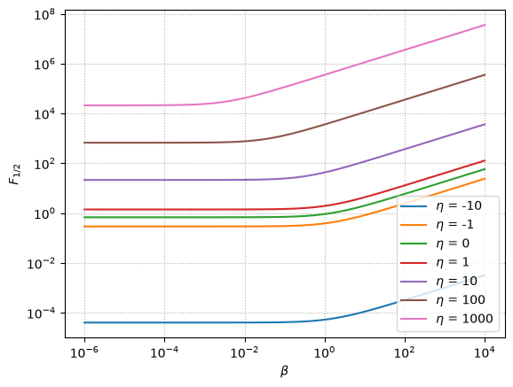
First, for fixed \(\eta\), let’s see the variation with \(\beta\)

k = 0.5
Fs = {}
betas = np.logspace(-6, 4, 50)
for eta in [-10, -1, 0,
            1, 10, 100, 1000]:
    res = []
    for beta in betas:
        F = pyna.FermiIntegral(k, eta, beta)
        F.evaluate(do_first_derivs=False, do_second_derivs=False)
        res.append(F.F)

    Fs[eta] = res

fig, ax = plt.subplots()
for key in Fs:
    ax.loglog(betas, Fs[key], label=rf"$\eta$ = {key}")
ax.legend()
ax.set_xlabel(r"$\beta$")
ax.set_ylabel(r"$F_{1/2}$")
ax.grid(ls=":")

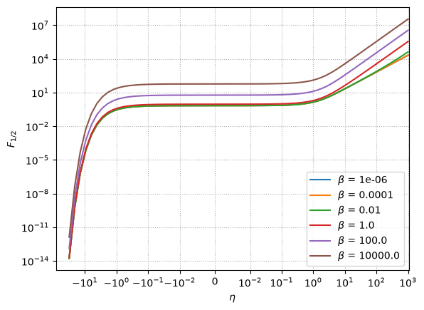
Now for fixed \(\beta\), let’s see the variation with \(\eta\).

etam = np.logspace(-2, 1.5, 21)
etap = np.logspace(-2, 3, 41)
etas = np.concatenate((-etam[::-1], etap))

k = 0.5
Fs = {}
for beta in np.logspace(-6, 4, 6):
    res = []
    for eta in etas:
        F = pyna.FermiIntegral(k, eta, beta)
        F.evaluate(do_first_derivs=False, do_second_derivs=False)
        res.append(F.F)

    Fs[beta] = res

fig, ax = plt.subplots()
for key in Fs:
    ax.plot(etas, Fs[key], label=rf"$\beta$ = {key}")
ax.legend()
ax.set_yscale("log")
ax.set_xscale("symlog", linthresh=1.e-2)
ax.set_xlabel(r"$\eta$")
ax.set_ylabel(r"$F_{1/2}$")
ax.grid(ls=":")