The Electron-Positron EOS#
The ElectronEOS class managed an electron-positron equation of state, including the effects of relativity and degeneracy. It does this by directly computing the necessary Fermi-Dirac integrals.
Warning
The ElectronEOS can be slow because it is solving for the degeneracy parameter,
\(\eta\), and doing all of the integrals at high precision.
Here we’ll explore the degeneracy parameter, \(\eta = (\mu - m_e c^2)/ (kT)\), where \(\mu\) is the chemical potential, as well as positron creation at low densities and high temperature.
import pynucastro as pyna
import numpy as np
Once we create an ElectronEOS, we can access the thermodynamics via the
pe_state function.
eos = pyna.eos.ElectronEOS()
We’ll create a grid of temperature and density and compute the thermodynamic quantities at each point.
Ts = np.logspace(4, 9, 26)
rhos = np.logspace(-4, 9, 66)
eta = np.zeros((len(rhos), len(Ts)))
n_e = np.zeros((len(rhos), len(Ts)))
n_pos = np.zeros((len(rhos), len(Ts)))
The only role composition plays in this EOS is determining the number density of electrons (assuming full ionization) via \(Y_e\).
comp = pyna.Composition(["he4"])
comp.set_equal()
The pe_state() function returns two EOSState objects—one for electrons and the other for positrons.
for ir, rho in enumerate(rhos):
    for it, T in enumerate(Ts):
        es, ps = eos.pe_state(rho, T, comp, compute_derivs=False)
        eta[ir, it] = es.eta
        n_e[ir, it] = es.n
        n_pos[ir, it] = ps.n
Now we’ll make some plots
import matplotlib.pyplot as plt
from matplotlib import colors
Degeneracy parameter#
First, the degeneracy parameter. Since our grid of EOS points was coarse, we’ll use some interpolation to smooth it.
fig = plt.figure(constrained_layout=True)
ax = fig.add_subplot(111)
im = ax.imshow(eta.T, origin="lower",
               norm=colors.SymLogNorm(linthresh=0.01, vmin=-eta.max(), vmax=eta.max()),
               extent=[np.log10(rhos.min()), np.log10(rhos.max()),
                       np.log10(Ts.min()), np.log10(Ts.max())],
               interpolation="bilinear",
               cmap="RdBu")
ax.set_xlabel(r"$\log_{10}(\rho)$")
ax.set_ylabel(r"$\log_{10}(T)$")
ax.set_title(r"$\eta$")
fig.colorbar(im, ax=ax, orientation="horizontal")
<matplotlib.colorbar.Colorbar at 0x7f8db992b0e0>
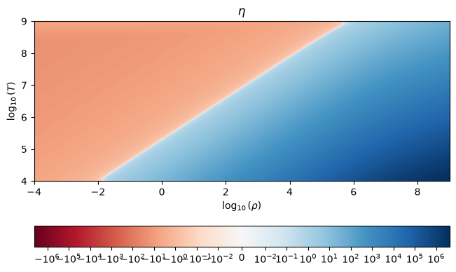
We see that at high temperatures, low densities, we are an idea gas (\(\eta \ll -1\)), while at high densities and low temperatures, we are very degenerate (\(\eta \gg 1\))
Electron-positron pairs#
At low density and very high temperatures (\(kT \sim m_e c^2\)), we can create electron positron pairs. Here we plot the fraction of positrons to the total number of electrons and positrons.
y = (n_pos / (n_pos + n_e))
y.min(), y.max()
(np.float64(0.0), np.float64(0.499999986135348))
fig = plt.figure(constrained_layout=True)
ax = fig.add_subplot(111)
im = ax.imshow(y.T, origin="lower",
               norm=colors.SymLogNorm(linthresh=1.e-5, vmin=1.e-50, vmax=0.5, clip=True),
               extent=[np.log10(rhos.min()), np.log10(rhos.max()),
                       np.log10(Ts.min()), np.log10(Ts.max())],
               interpolation="bilinear")
ax.set_xlabel(r"$\log_{10}(\rho)$")
ax.set_ylabel(r"$\log_{10}(T)$")
ax.set_title(r"$n^+ / (n^- + n^+)$")
fig.colorbar(im, ax=ax, orientation="horizontal")
<matplotlib.colorbar.Colorbar at 0x7f8db96dfcb0>
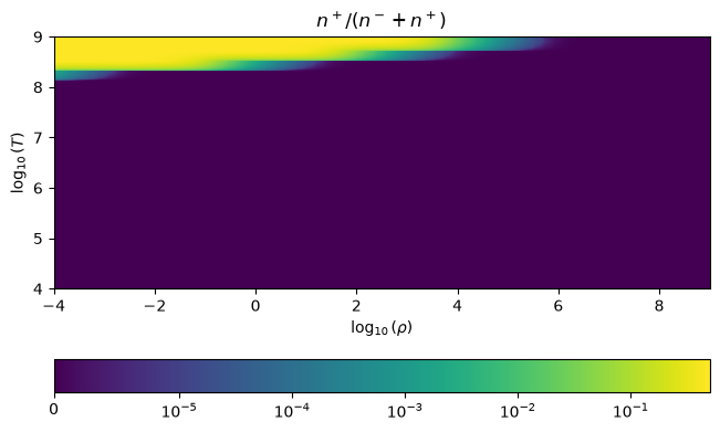
We see that we have nearly equal numbers of electrons and positrons at very low densities and high temperatures.