Integrating Networks with Temperature Evolution

So far, when integrating a reaction network in python, we’ve been solving

\[\frac{d{\bf Y}}{dt} = {\bf f}({\bf Y})\]

where \({\bf f}({\bf Y})\) is provided by the PythonNetwork rhs() function that is generated by write_network.

Now we want to instead solve the system:

\[\frac{d{\bf Y}}{dt} = {\bf f}(T, {\bf Y})\]

\[\frac{dT}{dt} = \frac{\epsilon(T, {\bf Y})}{c_x}\]

where \(\epsilon\) is the specific energy generation rate from the network and \(c_x\) is a specific heat (usually volume or pressure, depending on the application).

Note

The rhs and jacobian functions produced by write_network do not include temperature evolution, so we will need to wrap the rhs function and have the integrator approximate the Jacobian via differencing.

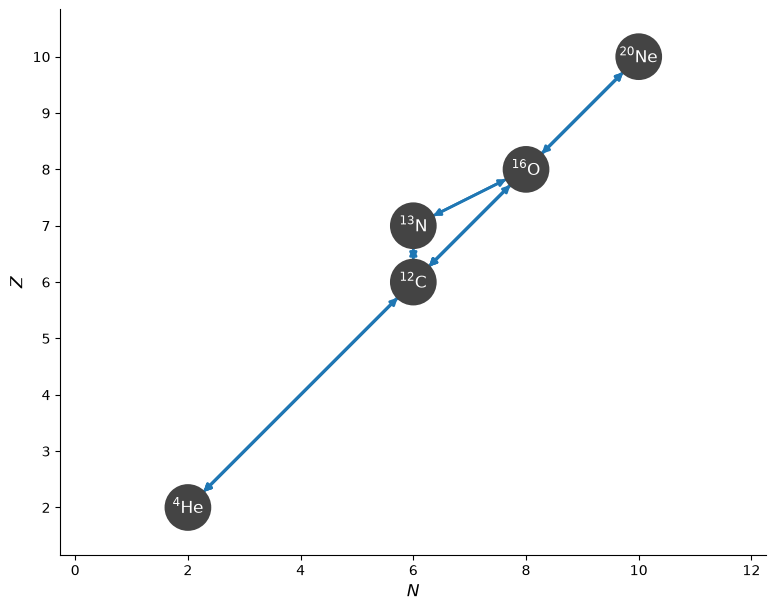
Let’s start with a simple He-burning network.

import pynucastro as pyna

net = pyna.network_helper(["p", "he4", "c12", "n13", "o16", "ne20"])

warning: C12 was not able to be linked in TabularLibrary
warning: He4 was not able to be linked in TabularLibrary
warning: p was not able to be linked in TabularLibrary
warning: O16 was not able to be linked in TabularLibrary
warning: N13 was not able to be linked in TabularLibrary
warning: Ne20 was not able to be linked in TabularLibrary

fig = net.plot()

No temperature evolution

First we’ll integrate without evolving the temperature.

from scipy.integrate import solve_ivp
import numpy as np

rho = 1.e5
T = 2.e8

comp = pyna.Composition(net.unique_nuclei)
comp.X[pyna.Nucleus("he4")] = 1
comp.normalize()
Y0 = np.array(list(comp.get_molar().values()))

tmax = 1.e7

net.write_network("henet.py")
import henet

/opt/hostedtoolcache/Python/3.14.2/x64/lib/python3.14/site-packages/pynucastro/rates/derived_rate.py:117: UserWarning: C12 partition function is not supported by tables: set pf = 1.0 by default
  warnings.warn(UserWarning(f'{nuc} partition function is not supported by tables: set pf = 1.0 by default'))
/opt/hostedtoolcache/Python/3.14.2/x64/lib/python3.14/site-packages/pynucastro/rates/derived_rate.py:117: UserWarning: N13 partition function is not supported by tables: set pf = 1.0 by default
  warnings.warn(UserWarning(f'{nuc} partition function is not supported by tables: set pf = 1.0 by default'))

sol = solve_ivp(henet.rhs, [0, tmax], Y0, method="BDF", jac=henet.jacobian,
                dense_output=True, args=(rho, T), rtol=1.e-6, atol=1.e-6)

import matplotlib.pyplot as plt

fig, ax = plt.subplots()

for i in range(henet.nnuc):
    ax.loglog(sol.t, sol.y[i,:] * henet.A[i], label=f"X({henet.names[i].capitalize()})")

ax.set_ylim(1.e-6, 1.1)
ax.legend(fontsize="small")
ax.set_xlabel("t (s)")
ax.set_ylabel("X")
ax.grid(ls=":")

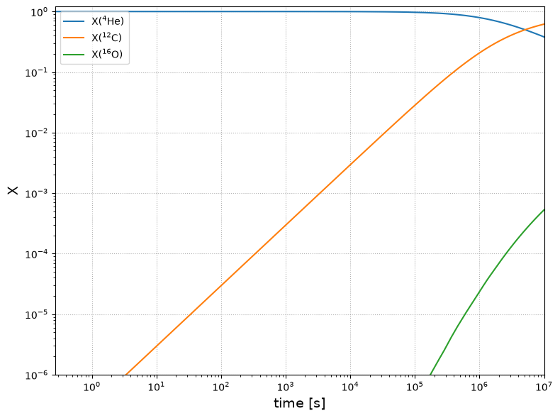
We see it takes about \(10^6\) s for the He mass fraction to start to deplete significantly.

Evolving temperature

We’ll call our vector of unknowns \(\xi = ({\bf Y}, T)\).

Now we’ll write our wrapper that computes \(d\xi/dt\), leveraging the network module we created with {\tt write_network}. In fact, we’ll pass that module into rhs_new as an argument, so we can easily use what’s needed from it.

Inside this function, we’ll call the EOS each time to get the updated specific heat.

def rhs_new(t, xi, pynet, rho):

    # unpack the incoming xi
    nspec = len(xi) - 1
    Y = xi[0:nspec]
    T = xi[-1]
    
    dxidt = np.zeros_like(xi)

    # first get the dYdt from our network module
    dxidt[0:nspec] = pynet.rhs(t, Y, rho, T)

    # now get the energy generation rate using this dY/dt
    eps = pynet.energy_release(dxidt[0:nspec])

    # use the EOS to get the specific heat
    eos = pyna.StellarEOS()
    comp = pynet.to_composition(Y)
    state = eos.pe_state(rho, T, comp)

    # and finally compute dT/dt
    dxidt[-1] = eps / state.c_v

    return dxidt
    

Now we’ll integrate this new system. We need to pass in both the network module and density are args, but we no longer pass temperature this way, since it is now one of the dependent variables in the ODE system.

xi0 = np.append(Y0, T)
sol2 = solve_ivp(rhs_new, [0, tmax], xi0, method="BDF",
                dense_output=True, args=(henet, rho), rtol=1.e-6, atol=1.e-6)

Now we can visualize. First the composition.

fig, ax = plt.subplots()

for i in range(henet.nnuc):
    ax.loglog(sol2.t, sol2.y[i,:] * henet.A[i], label=f"X({henet.names[i].capitalize()})")

ax.set_ylim(1.e-6, 1.1)
ax.legend(fontsize="small")
ax.set_xlabel("t (s)")
ax.set_ylabel("X")
ax.grid(ls=":")

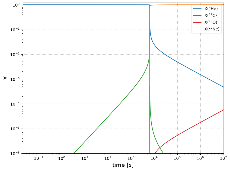
This looks dramatically different than the fixed-temperature case. This is not too surprising, since at these temperatures, the 3-\(\alpha\) rate is very temperature sensitive, so as the temperature increases due to the energy release from burning, the He burning rate increases dramatically.

fig, ax = plt.subplots()
ax.semilogx(sol2.t, sol2.y[-1,:])
ax.set_xlabel("t (s)")
ax.set_ylabel("T (K)")
ax.grid(ls=":")

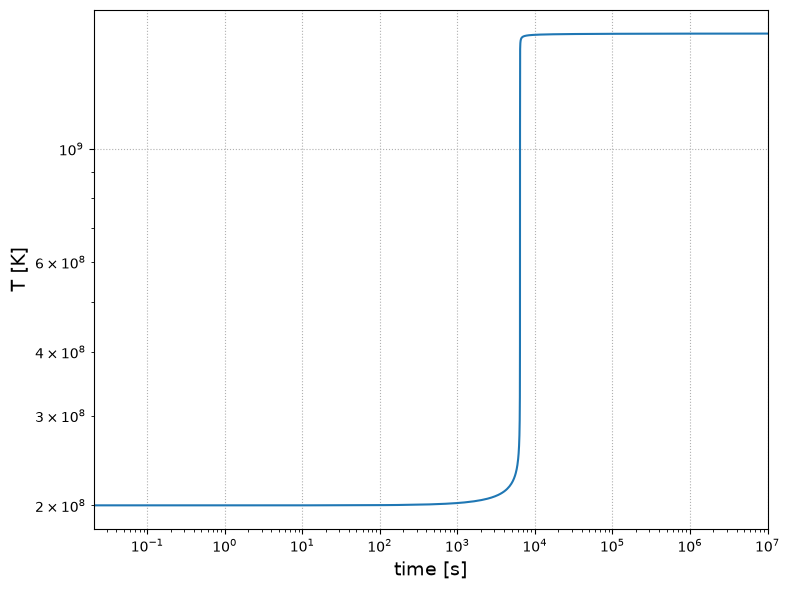
We see that the temperature increased from \(2\times 10^8\) K to over \(1.6\times 10^9\) K.

Caution

In a real star, this energy release would drive a hydrodynamic flow which, depending on the timescale of the energy release vs. sound waves, could drive an expansive flow and quench some of this heating. To really capture this, a full hydrodynamics calculation is needed.

Tip

It is straightforward to include thermal neutrino loses in the temperature evolution equation as well, using the sneut5 method.