The “aprox13” network

The aprox13 network is widely used for explosive He burning in multidimensional simulations. It has 2 main approximations:

• C+C, C+O, and O+O burning are simplified, removing the intermediate nucleus from the proton emission branch and neglecting the neutron-emission branch

• The \((\alpha,p)(p,\gamma)\) links are combined with \((\alpha,\gamma)\)

We can do both approximations.

A starting network

To begin, we’ll create a network will all of the nuclei (including those that will be approximated out later). We’ll use network_helper so we automatically rederive reverse rates using detailed balance.

import pynucastro as pyna

net = pyna.network_helper(["p", "he4",
                           "c12", "o16", "ne20", "na23",
                           "mg24", "al27", "si28", "p31", "s32",
                           "cl35", "ar36", "k39", "ca40",
                           "sc43", "ti44", "v47", "cr48",
                           "mn51", "fe52", "co55", "ni56"])

warning: C12 was not able to be linked in TabularLibrary
warning: Al27 was not able to be linked in TabularLibrary
warning: S32 was not able to be linked in TabularLibrary
warning: Cr48 was not able to be linked in TabularLibrary
warning: Si28 was not able to be linked in TabularLibrary
warning: Sc43 was not able to be linked in TabularLibrary
warning: Ti44 was not able to be linked in TabularLibrary
warning: Na23 was not able to be linked in TabularLibrary
warning: K39 was not able to be linked in TabularLibrary
warning: Co55 was not able to be linked in TabularLibrary
warning: Mg24 was not able to be linked in TabularLibrary
warning: He4 was not able to be linked in TabularLibrary
warning: Ca40 was not able to be linked in TabularLibrary
warning: Cl35 was not able to be linked in TabularLibrary
warning: Ne20 was not able to be linked in TabularLibrary
warning: Ni56 was not able to be linked in TabularLibrary
warning: P31 was not able to be linked in TabularLibrary
warning: Ar36 was not able to be linked in TabularLibrary
warning: Mn51 was not able to be linked in TabularLibrary
warning: p was not able to be linked in TabularLibrary
warning: Fe52 was not able to be linked in TabularLibrary
warning: O16 was not able to be linked in TabularLibrary
warning: V47 was not able to be linked in TabularLibrary

fig = net.plot(rotated=True, hide_xalpha=True,
               size=(1200, 300), node_size=600, node_font_size=10)

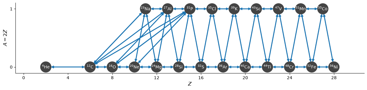
net.summary()

Network summary
---------------
  explicitly carried nuclei: 23
  approximated-out nuclei: 0
  inert nuclei (included in carried): 0

  total number of rates: 92

  rates explicitly connecting nuclei: 92
  hidden rates: 0

  reaclib rates: 46
  starlib rates: 0
  temperature tabular rates: 0
  weak tabular rates: 0
  approximate rates: 0
  derived rates: 46
  modified rates: 0
  custom rates: 0

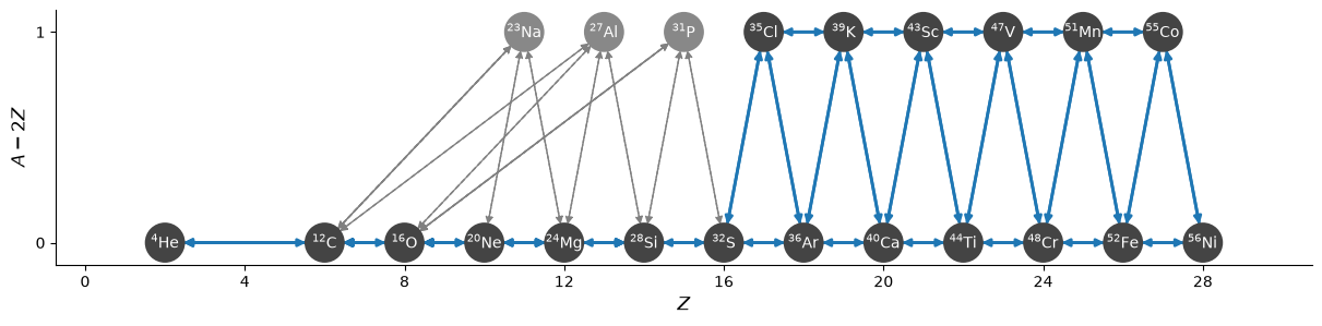
Approximating

Now we’ll approximate the C/O burning

from pynucastro.rates.aprox_family_rates import make_CO_approx_rates

approx_net = pyna.PythonNetwork(rates=net.get_rates())

approx_net.make_CO_burning_approx("C")
approx_net.remove_nuclei(["na23"])

approx_net.make_CO_burning_approx("CO")
approx_net.remove_nuclei(["al27"])

approx_net.make_CO_burning_approx("O")
approx_net.remove_nuclei(["p31"])

fig = approx_net.plot(rotated=True, hide_xalpha=True,
                      size=(1200, 300), node_size=600, node_font_size=10)

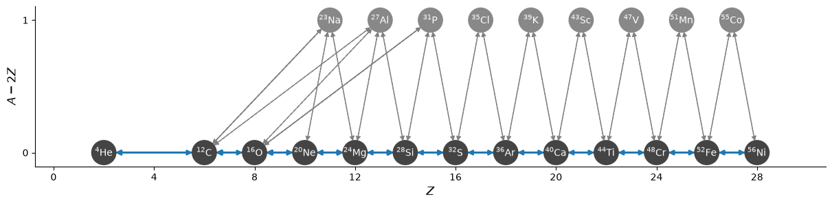
now the \((\alpha,p)(p,\gamma)\) approximation

approx_net.make_ap_pg_approx(intermediate_nuclei=["cl35", "k39", "sc43", "v47", "mn51", "co55"])
approx_net.remove_nuclei(["cl35", "k39", "sc43", "v47", "mn51", "co55"])

fig = approx_net.plot(rotated=True, hide_xalpha=True,
                      size=(1200, 300), node_size=600, node_font_size=10)

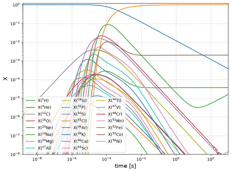
Comparing the integration

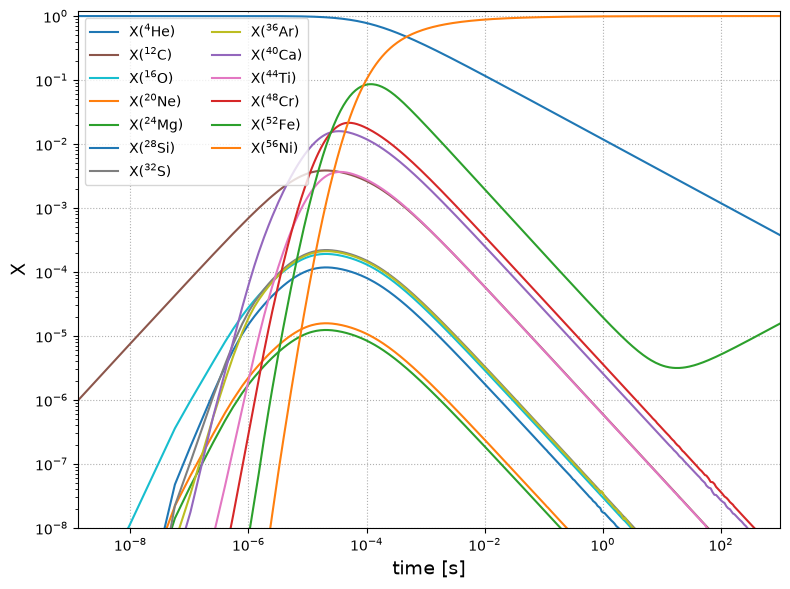
the full network

net.write_network("full_aprox13.py")
import full_aprox13 as fn

/opt/hostedtoolcache/Python/3.14.4/x64/lib/python3.14/site-packages/pynucastro/rates/derived_rate.py:120: UserWarning: C12 partition function is not supported by tables: set log_pf = 0.0 by default
  warnings.warn(UserWarning(f'{nuc} partition function is not supported by tables: set log_pf = 0.0 by default'))

rho = 1.e7
T = 3.e9

comp = pyna.Composition(net.unique_nuclei)
comp.X[pyna.Nucleus("he4")] = 1.0
Y0 = list(comp.get_molar().values())

tmax = 1000.0

sol_full = net.integrate_network(tmax, rho, T, Y0, rtol=1.e-6)

fig = sol_full.plot_evolution(ymin=1.e-8)

/opt/hostedtoolcache/Python/3.14.4/x64/lib/python3.14/site-packages/pynucastro/networks/python_network.py:379: UserWarning: Attempt to set non-positive xlim on a log-scaled axis will be ignored.
  ax.set_xlim(tmin, tmax)

aprox13 net

comp = pyna.Composition(approx_net.unique_nuclei)
comp.X[pyna.Nucleus("he4")] = 1.0
Y0 = list(comp.get_molar().values())

sol_approx = approx_net.integrate_network(tmax, rho, T, Y0, rtol=1.e-6)

/opt/hostedtoolcache/Python/3.14.4/x64/lib/python3.14/site-packages/pynucastro/rates/derived_rate.py:120: UserWarning: C12 partition function is not supported by tables: set log_pf = 0.0 by default
  warnings.warn(UserWarning(f'{nuc} partition function is not supported by tables: set log_pf = 0.0 by default'))

fig = sol_approx.plot_evolution(ymin=1.e-8)

/opt/hostedtoolcache/Python/3.14.4/x64/lib/python3.14/site-packages/pynucastro/networks/python_network.py:379: UserWarning: Attempt to set non-positive xlim on a log-scaled axis will be ignored.
  ax.set_xlim(tmin, tmax)

Comparing

import matplotlib.pyplot as plt

fig, ax = plt.subplots()

for i, nuc in enumerate(sol_approx.unique_nuclei):
    lw = 1
    if sol_approx.X[i, :].max() > 1.e-2:
        lw = 2
    ax.loglog(sol_approx.t, sol_approx.X[i, :],
              linestyle=":", color=f"C{i}", lw=lw)    
    idx = sol_full.unique_nuclei.index(nuc)
    ax.loglog(sol_full.t, sol_full.X[idx, :],
              label=rf"X$({nuc.pretty})$",              
              linestyle="-", color=f"C{i}", lw=lw)

ax.set_ylim(1.e-6, 1.1)
ax.set_xlim(1.e-10, 100)
fig.set_size_inches((8,6))
ax.set_xlabel("time (s)")
ax.set_ylabel("X")
ax.legend(ncol=2)
ax.grid()

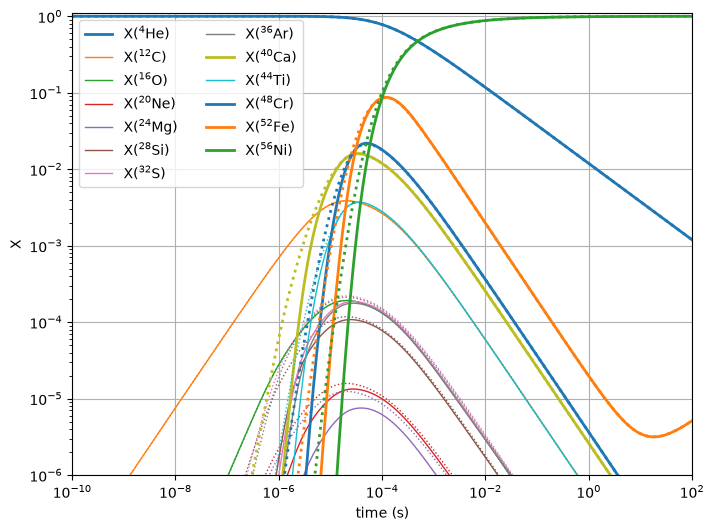
We see good agreement for the nuclei the two networks have in common.