Effects of Thermal Neutrino Cooling in Network Integrations

We will compare two one-zone, self-heating integrations of the same He-burning network: one without thermal neutrino cooling and one with thermal neutrino cooling enabled.

When integrate_network is run with self_heating=True, adding thermal_neutrinos=True changes the temperature equation to

\[ \frac{dT}{dt} = \frac{\epsilon_\mathrm{nuc} - \epsilon_\nu}{c_V}, \]

where \(\epsilon_\mathrm{nuc}\) is the nuclear energy generation rate, \(\epsilon_\nu\) is evaluated with sneut5, and \(c_V\) is the specific heat from the equation of state.

Note

This is a one-zone calculation. It does not include hydrodynamic expansion or transport, so it is intended to demonstrate how the cooling term enters the network integration rather than to model a full stellar environment.

Network Setup

import matplotlib.pyplot as plt
import pynucastro as pyna

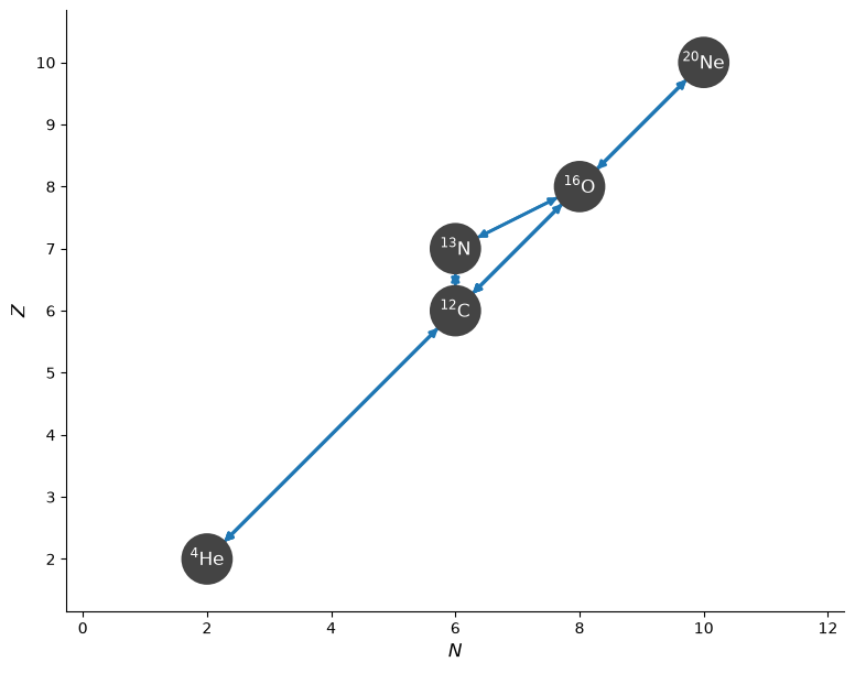
We use a small He-burning network and initialize the zone with pure \(^4\mathrm{He}\).

net = pyna.network_helper(["p", "he4", "c12", "n13", "o16", "ne20"])
fig = net.plot()

rho = 1.e5
T = 2.e8

comp = pyna.Composition(net.unique_nuclei)
comp.X[pyna.Nucleus("he4")] = 1
comp.normalize()
Y0 = comp.get_molar_array()

tmax = 1.e7

First we integrate with self-heating, but without thermal neutrino cooling.

sol_no_cooling = net.integrate_network(tmax, rho, T, Y0,
                                       self_heating=True,
                                       rtol=1.e-6, atol=1.e-6)

/opt/hostedtoolcache/Python/3.14.6/x64/lib/python3.14/site-packages/pynucastro/rates/derived_rate.py:125: UserWarning: C12 partition function is not supported by tables: set log_pf = 0.0 by default
  warnings.warn(UserWarning(f'{nuc} partition function is not supported by tables: set log_pf = 0.0 by default'))
/opt/hostedtoolcache/Python/3.14.6/x64/lib/python3.14/site-packages/pynucastro/rates/derived_rate.py:125: UserWarning: N13 partition function is not supported by tables: set log_pf = 0.0 by default
  warnings.warn(UserWarning(f'{nuc} partition function is not supported by tables: set log_pf = 0.0 by default'))

Now we repeat the integration with thermal_neutrinos=True. This evaluates sneut5 along the trajectory and subtracts the neutrino loss rate from the nuclear energy generation rate in the temperature equation.

sol_cooling = net.integrate_network(tmax, rho, T, Y0,
                                    self_heating=True,
                                    thermal_neutrinos=True,
                                    rtol=1.e-6, atol=1.e-6)

/opt/hostedtoolcache/Python/3.14.6/x64/lib/python3.14/site-packages/pynucastro/rates/derived_rate.py:125: UserWarning: C12 partition function is not supported by tables: set log_pf = 0.0 by default
  warnings.warn(UserWarning(f'{nuc} partition function is not supported by tables: set log_pf = 0.0 by default'))
/opt/hostedtoolcache/Python/3.14.6/x64/lib/python3.14/site-packages/pynucastro/rates/derived_rate.py:125: UserWarning: N13 partition function is not supported by tables: set log_pf = 0.0 by default
  warnings.warn(UserWarning(f'{nuc} partition function is not supported by tables: set log_pf = 0.0 by default'))

Energy Generation and Neutrino Loss

For the cooled trajectory, we can compare the nuclear energy generation rate, \(\epsilon_\mathrm{nuc}\), with the thermal neutrino loss rate, \(\epsilon_\nu\).

fig = sol_cooling.plot_energy_generation(ymax=1.e18,
                                         include_neutrino_loss=True)

/opt/hostedtoolcache/Python/3.14.6/x64/lib/python3.14/site-packages/pynucastro/networks/python_network.py:615: UserWarning: Attempt to set non-positive xlim on a log-scaled axis will be ignored.
  ax.set_xlim(tmin, tmax)

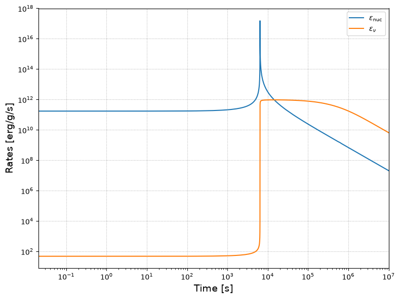
During the runaway, \(\epsilon_\mathrm{nuc}\) is much larger than \(\epsilon_\nu\). After the peak, the nuclear energy generation rate falls while the neutrino loss rate remains large for longer.

Temperature Evolution

The effect of the loss term is visible by comparing the temperature histories from the two integrations.

fig, ax = plt.subplots()

mask_no_cooling = sol_no_cooling.t > 0
mask_cooling = sol_cooling.t > 0

ax.loglog(sol_no_cooling.t[mask_no_cooling],
          sol_no_cooling.Temp[mask_no_cooling],
          label="without neutrino cooling")
ax.loglog(sol_cooling.t[mask_cooling],
          sol_cooling.Temp[mask_cooling],
          label="with neutrino cooling")

ax.set_xlabel("Time [s]")
ax.set_ylabel("T [K]")
ax.legend()
ax.grid(ls=":")
fig.tight_layout()

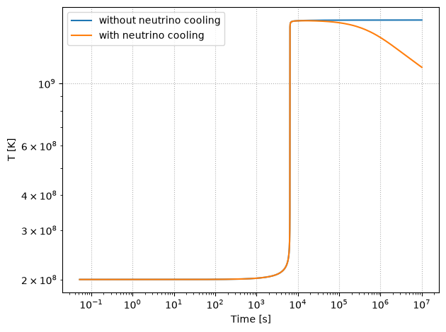
The integration with thermal neutrino cooling cools after the runaway, while the integration without this loss term remains hot. The difference arises because the cooling term changes the temperature history, and the reaction rates depend on temperature.