MESA basic.net Network

The MESA stellar evolution code uses the basic.net network as a simple network for basic stellar evolution. basic.net use 8 nuclei to approximate pp, CNO (but not hot-CNO), and He burning. It also serves as the starting point for many other nets in MESA.

pynucastro can make a version of basic.net using ApproximateRate, BranchedRate, and ModifiedRate.

We will make three groups of approximations:

• pp-chains : we’ll leave out deuterium and approximate pp-II and pp-III

• CNO : we’ll approximate several rate sequences

• helium burning : we’ll focus only on the most important rates

We will also not include reverse rates explicitly.

import pynucastro as pyna

rl = pyna.ReacLibLibrary()

pp rates

We will make the following approximations:

• \(d\) is not evolved, so the sequences \(p(p,e^+\nu)d(p,\gamma){}^{3}\mathrm{He}\) and it’s electron capture equivalent are treated as a single rate. We’ll use ModifiedRate for this.

• The pp-II and pp-III chains are also approximated, via the rate sequences:

  • \({}^4{\rm He}({}^3{\rm He},\gamma){}^7{\rm Be}(e^-,\nu){}^7{\rm Li}(p,\alpha){}^4{\rm He}\)

  • \({}^4{\rm He}({}^3{\rm He},\gamma){}^7{\rm Be}(p,\gamma){}^8{\rm B}(,e^+\nu){}^8{\rm B}(,\alpha){}^4{\rm He}\)

  We could treat these as separate rates, using a BranchedRate on \({}^7\mathrm{Be}\) (although currently BranchedRate assumes that the reactants are the same for the branched). However, since these two branches have the same endpoint, we could just use a ModifiedRate. The only reason to treat them separately is if we want to account for the different neutrino energy loss in the two branches.

  Note

  Currently, pynucastro does not have a data source for these neutino energies, so they will not be accounted for.

• The remaining rates, \(^{3}{\rm He}(^{3}{\rm He},2p)^{4}{\rm He}\) and \({}^3{\rm He}(p,e^+\nu){}^4{\rm He}\) are just regular ReacLib rates.

Creating the rates

First we’ll create the rates involved in \(p + p\). There are actually two rates here from ReacLib–an electron capture and a \(\beta^+\)-decay. We will approximate them both by changing the endpoint to be \({}^3\mathrm{He}\) so the net reaction is \(3~p \rightarrow {}^3\mathrm{He}\):

When we do get_rate_by_name with "p(p,)d", we get a list of rates, which we unpack here:

rpp, rpep = rl.get_rate_by_name("p(p,)d")

rpp, rpep

(p + p ⟶ H2 + e⁺ + 𝜈, p + p + e⁻ ⟶ H2 + 𝜈)

Now we create ModifiedRate from these, adding a proton and changing the endpoint. Notice that we explicitly pass the rate_source from the underlying rates into the ModifiedRate creation—this is important in this case, because it will help distinguish the \(e^-\)-capture from the \(\beta^+\)-decay:

rppp_he3 = pyna.ModifiedRate(rpp,
                             new_products=[pyna.Nucleus("he3")],
                             stoichiometry={pyna.Nucleus("p"): 3},
                             description="p(p,e⁺ν)d(p,γ)He3",
                             rate_source=rpp.src)

rpepp_he3 = pyna.ModifiedRate(rpep,
                              new_products=[pyna.Nucleus("he3")],
                              stoichiometry={pyna.Nucleus("p"): 3},
                              description="p(pe⁻,ν)d(p,γ)He3",
                              rate_source=rpep.src)

rppp_he3, rpepp_he3

(3 p ⟶ He3 + e⁺ + 𝜈, 3 p + e⁻ ⟶ He3 + 𝜈)

The \({}^3\mathrm{He} + {}^3\mathrm{He}\) and \({}^3\mathrm{He} + p\) rates are unapproximated.

rhe3he3 = rl.get_rate_by_name("he3(he3,pp)he4")
rhe3p = rl.get_rate_by_name("he3(p,)he4")

For the \({}^{3}\mathrm{He} + {}^{4}\mathrm{He}\) rate, we need to consume a proton, but that should not factor into how the rate’s \(dY/dt\) term is constructed. We use the not_in_ydot_term functionality described in Rate Sequences with Extra Reactants.

rhe3he4 = rl.get_rate_by_name("he4(he3,g)be7")
rhe3he4p_2he4 = pyna.ModifiedRate(rhe3he4,
                                  new_reactants=[pyna.Nucleus("he4"),
                                                 pyna.Nucleus("he3"),
                                                 pyna.Nucleus("p")],
                                  new_products=[pyna.Nucleus("he4"),
                                                pyna.Nucleus("he4")],
                                  not_in_ydot_term=[pyna.Nucleus("p")],
                                  description="He4(He3,γ)Be7(e⁻,ν)Li7(p,α)He4")

We’ll create a library for the pp burning:

lib_pp = pyna.Library(rates=[rppp_he3, rpepp_he3,
                             rhe3he3, rhe3p, rhe3he4p_2he4])

CNO rates

We will use the approximation from BranchedRate. This approximates the sequences:

• \({}^{12}{\rm C}(p, \gamma){}^{13}{\rm N}(,e^+\nu){}^{13}{\rm C}(p,\gamma){}^{14}{\rm N}\)

• \({}^{14}{\rm N}(p, \gamma){}^{15}{\rm O}(,e^+\nu){}^{15}{\rm N}(p,\alpha){}^{12}{\rm C}\)

• \({}^{14}{\rm N}(p,\gamma){}^{15}{\rm O}(,e^+\nu){}^{15}{\rm N}(p,\gamma){}^{16}{\rm O}\)

• \({}^{16}{\rm O}(p,\gamma){}^{17}{\rm F}(,e^+\nu){}^{17}{\rm O}(p,\alpha){}^{14}{\rm N}\)

using BranchedRate or ModifiedRate.

Important

This will not capture hot-CNO, since it does not consider the \(\beta\)-limiting from \({}^{14}\mathrm{O}\) and \({}^{15}\mathrm{O}\). This is consistent with MESA’s basic.net.

Creating the rates

First we get the underlying rates for the CNO cycle

rc12pg = rl.get_rate_by_name("c12(p,g)n13")
rn14pg = rl.get_rate_by_name("n14(p,g)o15")
rn15pa = rl.get_rate_by_name("n15(p,a)c12")
rn15pg = rl.get_rate_by_name("n15(p,g)o16")
ro16pg = rl.get_rate_by_name("o16(p,g)f17")

Now we do the 4 rate approximations:

rc12_2p_n14 = pyna.ModifiedRate(rc12pg,
                                new_products=[pyna.Nucleus("n14")],
                                stoichiometry={pyna.Nucleus("p"): 2},
                                description="C12(p,γ)N13(,e⁺ν)C13(p,γ)N14")

rn14_2p_c12 = pyna.BranchedRate(rn14pg,
                                primary_branch=rn15pa,
                                other_branch=rn15pg,
                                stoichiometry={pyna.Nucleus("p"): 2},
                                description="N14(p,γ)O15(,e⁺ν)N15(p,α)C12")

rn14_2p_o16 = pyna.BranchedRate(rn14pg,
                                primary_branch=rn15pg,
                                other_branch=rn15pa,
                                stoichiometry={pyna.Nucleus("p"): 2},
                                description="N14(p,γ)O15(,e⁺ν)N15(p,γ)O16")

ro16_2p_n14_a = pyna.ModifiedRate(ro16pg,
                                  new_products=[pyna.Nucleus("n14"),
                                                pyna.Nucleus("he4")],
                                  stoichiometry={pyna.Nucleus("p"): 2},
                                  description="O16(p,γ)F17(,e⁺ν)O17(p,α)N14")

We’ll create a library for the CNO burning:

lib_cno = pyna.Library(rates=[rc12_2p_n14, rn14_2p_c12,
                              rn14_2p_o16, ro16_2p_n14_a])

He-burning

We will do a simple He burning presciption:

• We will include triple alpha

• For \({}^{12}\mathrm{C}(\alpha,\gamma){}^{16}\mathrm{O}\), we also include the alternate \({}^{12}{\rm C}(\alpha,p){}^{15}{\rm N}(p,\gamma){}^{16}{\rm O}\) using ApproximateRate

• We include the “3/2-\(\alpha\) capture onto \({}^{14}\mathrm{N}\) discussed in Modified Rates.

• Finally, we’ve add the \(\alpha\)-capture sequences:

  • \(^{16}{\rm O}(\alpha,\gamma)^{20}{\rm Ne}\) + \({}^{16}{\rm O}(\alpha,p){}^{19}{\rm F}(p,\gamma)^{20}{\rm Ne}\)

  • \(^{20}{\rm Ne}(\alpha,\gamma)^{24}{\rm Mg}\) + \(^{20}{\rm Ne}(\alpha,p){}^{23}{\rm Ne}(p,\gamma){}^{24}{\rm Mg}\)

  using ApproximateRate

Creating the rates

r3a = rl.get_rate_by_name("a(aa,g)c12")

rc12ag, _ = pyna.rates.make_ap_pg_rates(rl, "c12", "o16",
                                        use_detailed_balance=True)

rn14ag = rl.get_rate_by_name("n14(a,g)f18")
rn14ag_lite = pyna.ModifiedRate(rn14ag,
                                new_products=["ne20"],
                                stoichiometry={pyna.Nucleus("he4"): 1.5})

ro16ag, _ = pyna.rates.make_ap_pg_rates(rl, "o16", "ne20",
                                        use_detailed_balance=True)
rne20ag, _ = pyna.rates.make_ap_pg_rates(rl, "ne20", "mg24",
                                         use_detailed_balance=True)

Finally we will create a library:

lib_he = pyna.Library(rates=[r3a, rc12ag,
                             rn14ag_lite, ro16ag, rne20ag])

Constructing the network

We will construct the network using the three libraries we just created.

Note

Even though we have two rates that look like \(3~p \rightarrow {}^3\mathrm{He}\), they are distinguishable by their weak rate type, and this will not raise a RateDuplicationError.

net = pyna.PythonNetwork(libraries=[lib_pp, lib_cno, lib_he])

net.summary()

Network summary
---------------
  explicitly carried nuclei: 8
  approximated-out nuclei: 3
  inert nuclei (included in carried): 0

  NSE compatible? False

  total number of rates: 39

  rates explicitly connecting nuclei: 14
  hidden rates: 25

  reaclib rates: 19
  starlib rates: 0
  temperature tabular rates: 0
  weak tabular rates: 0
  approximate rates: 3
  derived rates: 9
  branched rates: 2
  modified rates: 6
  custom rates: 0

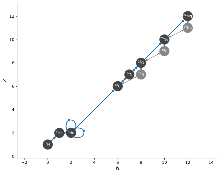
fig = net.plot(always_show_p=True, node_size=550, node_font_size="9")

Integrating

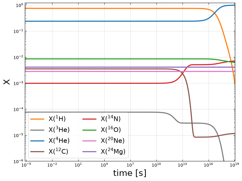
In a star, we will have H core burning, followed by contraction, and then He core burning. The thermodynamic conditions at these two stages will differ quite a bit. So we’ll test out this network by doing two burns (one after another).

First, H burning. We’ll choose conditions similar to the Sun

rho = 150
T = 1.5e7
comp = pyna.Composition(net.unique_nuclei, init="solar")

tmax = 1.e23

We will burn until H exhaustion.

sol = net.integrate_network(tmax, rho, T, comp,
                            stopping_condition=("h1", 1.e-3))

/opt/hostedtoolcache/Python/3.14.7/x64/lib/python3.14/site-packages/pynucastro/rates/derived_rate.py:125: UserWarning: C12 partition function is not supported by tables: set log_pf = 0.0 by default
  warnings.warn(UserWarning(f'{nuc} partition function is not supported by tables: set log_pf = 0.0 by default'))
/opt/hostedtoolcache/Python/3.14.7/x64/lib/python3.14/site-packages/pynucastro/rates/derived_rate.py:125: UserWarning: N15 partition function is not supported by tables: set log_pf = 0.0 by default
  warnings.warn(UserWarning(f'{nuc} partition function is not supported by tables: set log_pf = 0.0 by default'))

fig = sol.plot_evolution(ymin=1.e-6)

/opt/hostedtoolcache/Python/3.14.7/x64/lib/python3.14/site-packages/pynucastro/networks/python_network.py:496: UserWarning: Attempt to set non-positive xlim on a log-scaled axis will be ignored.
  ax.set_xlim(tmin, tmax)

Now we’ll take this composition as the starting point for He burning, but use a higher density and temperature, corresponding to the Sun’s conditions on the horizontal branch

X_final = sol.X[:, -1]
comp.set_array(X_final)

T = 1.e8
rho = 20000

sol2 = net.integrate_network(tmax, rho, T, comp,
                             stopping_condition=("he4", 1.e-3))

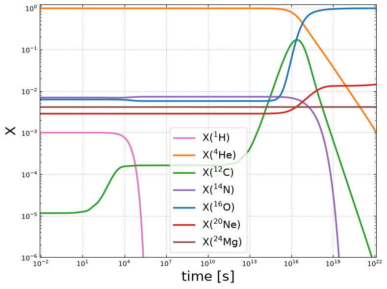
fig = sol2.plot_evolution(ymin=1.e-6)