Importing MESA Models and Visualizing Reactive Flow

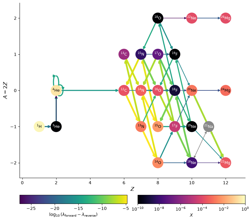
We can visualize the reactive flow through MESA stellar evolution models by reconstructing the network and using pynucastro’s machinery to evaluate the rates.

We leverage mesa_reader for loading the MESA data.

import mesa_reader as mr

We’ll start with a MESA model for a classical nova. This is from the MESA test suite ($MESA_DIR/star/test_suite/wd_nova_burst. We’ll use the model file closest to peak luminosity.

model = mr.MesaData("mesa_nova_profile8.data")

mesa_utils

The pynucastro mesa_utils module will read in the data and convert it to pynucastro types.

from pynucastro import mesa_utils
import pynucastro as pyna

mesa_zones = mesa_utils.MesaModel(model)

We can use the methods in MesaModel to access the data in various ways.

For example, we can get the zone corresponding to peak temperature:

idx = mesa_zones.get_peak_index("T")
idx

np.int64(570)

Reproducing the network

MESA has many different reaction networks, which often have different rate approximations. We could just find all of the nuclei used in the simulation, via:

nuclei = mesa_utils.get_nuclei(model)

and then build a network using network_helper, but that will not automatically reproduce the approximations, if any were used.

From within a MESA simulation, you can output all of the reaction rates used by adding:

show_net_reactions_info = .true.

to the &star_job inline.

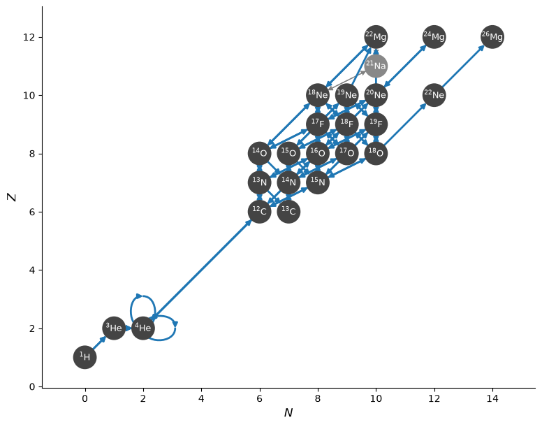
In our case, the nova run was built using the cno_extras_o18_to_mg26_plus_fe56.net network. This is essentially our cno networks with the addition of \({}^{22}\mathrm{Ne}\) and \({}^{26}\mathrm{Mg}\). So we can build the network from there.

net = pyna.common_networks.cno()

rl = pyna.ReacLibLibrary()
ro18ag = rl.get_rate_by_name("o18(a,g)ne22")
rne22ag = rl.get_rate_by_name("ne22(a,g)mg26")

net.add_rates([ro18ag, rne22ag])

fig = net.plot(node_size=500, node_font_size="9",
               always_show_p=True)

Visualizing the reactive flow

We can use MesaModel.get_zone_data to get the data corresponding to a single MESA zone (it will be returned as a MesaZoneState object.

We’ll use the index corresponding to peak \(T\) that we found above.

state = mesa_zones.get_zone_data(idx)

fig = net.plot(state.rho, state.T, state.comp,
               always_show_p=True,
               rotated=True,
               use_net_rate=True,
               size=(800, 700),
               node_size=550, node_font_size=9,
               color_nodes_by_abundance=True)

/opt/hostedtoolcache/Python/3.14.7/x64/lib/python3.14/site-packages/pynucastro/rates/derived_rate.py:125: UserWarning: C12 partition function is not supported by tables: set log_pf = 0.0 by default
  warnings.warn(UserWarning(f'{nuc} partition function is not supported by tables: set log_pf = 0.0 by default'))
/opt/hostedtoolcache/Python/3.14.7/x64/lib/python3.14/site-packages/pynucastro/rates/derived_rate.py:125: UserWarning: N13 partition function is not supported by tables: set log_pf = 0.0 by default
  warnings.warn(UserWarning(f'{nuc} partition function is not supported by tables: set log_pf = 0.0 by default'))
/opt/hostedtoolcache/Python/3.14.7/x64/lib/python3.14/site-packages/pynucastro/rates/derived_rate.py:125: UserWarning: C13 partition function is not supported by tables: set log_pf = 0.0 by default
  warnings.warn(UserWarning(f'{nuc} partition function is not supported by tables: set log_pf = 0.0 by default'))
/opt/hostedtoolcache/Python/3.14.7/x64/lib/python3.14/site-packages/pynucastro/rates/derived_rate.py:125: UserWarning: N14 partition function is not supported by tables: set log_pf = 0.0 by default
  warnings.warn(UserWarning(f'{nuc} partition function is not supported by tables: set log_pf = 0.0 by default'))
/opt/hostedtoolcache/Python/3.14.7/x64/lib/python3.14/site-packages/pynucastro/rates/derived_rate.py:125: UserWarning: N15 partition function is not supported by tables: set log_pf = 0.0 by default
  warnings.warn(UserWarning(f'{nuc} partition function is not supported by tables: set log_pf = 0.0 by default'))